How to Drill and Construct Deep Water Borehole
After Drill-Rig Setup, connect the discharge piping. Depending on the type of drilling operation, connect either the air compressor or
Read MorePROJECT GUIDE & IN-DEPTH REVIEW
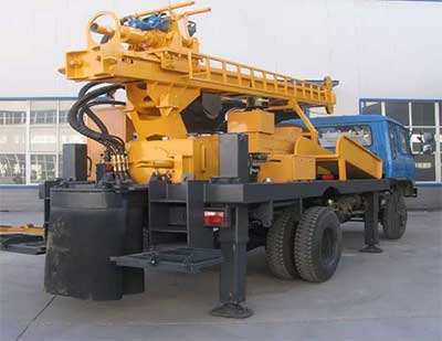
After Drill-Rig Setup, connect the discharge piping. Depending on the type of drilling operation, connect either the air compressor or
Read More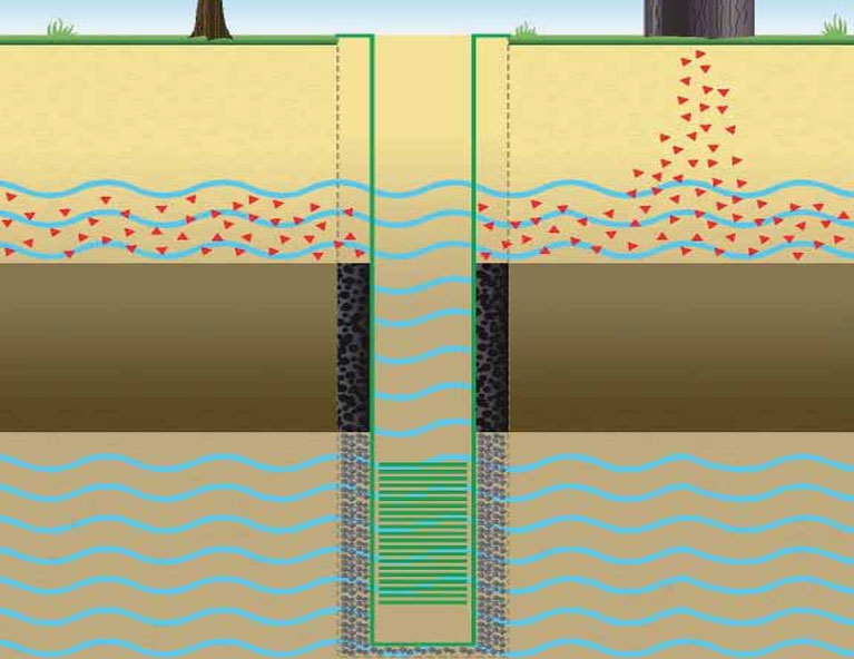
To achieve a good well design, a drilling log should be completed, a drilling log during the actual drilling process,
Read More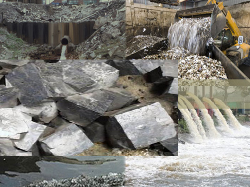
Ground water is a resource found under the earth’s surface. Most ground water comes from rain and melting snow soaking
Read More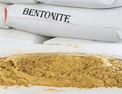
Drilling mud, also called drilling fluid is use for water borehole drilling. Drilling mud is pumped down the hollow drill
Read More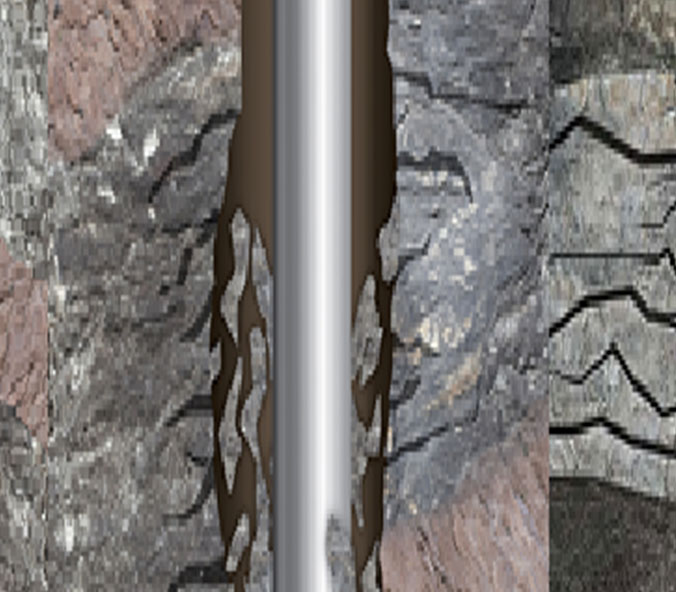
A lack of accurate pore-pressure prediction and wellbore stability analysis can result in unscheduled drilling events, such as blowouts, kicks,
Read More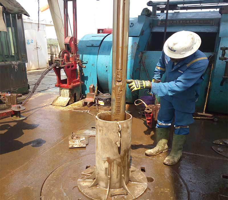
Consultant wellsite geologists, in the oil and gas industry, provide contract services to clients by bringing skill and experience in
Read More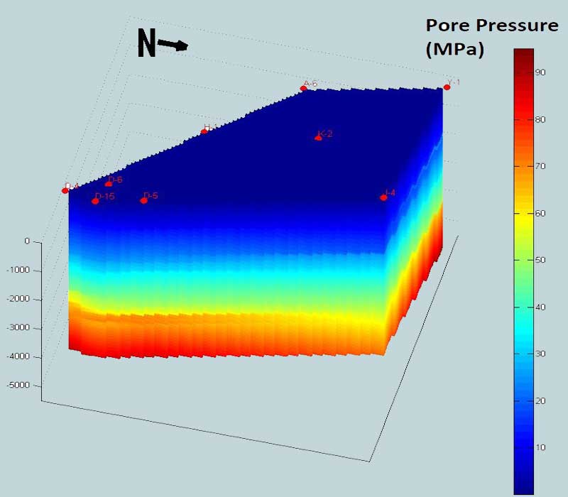
Our pore pressure computer program (Geopressure software) for detection / analysis of abnormal pore pressures during mud logging (drilling) operation
Read More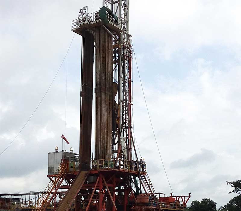
Qualitative Pressure detection When abnormal pore pressures are not accurately predicted in pre-drill stage or detected in real-time drilling, it
Read More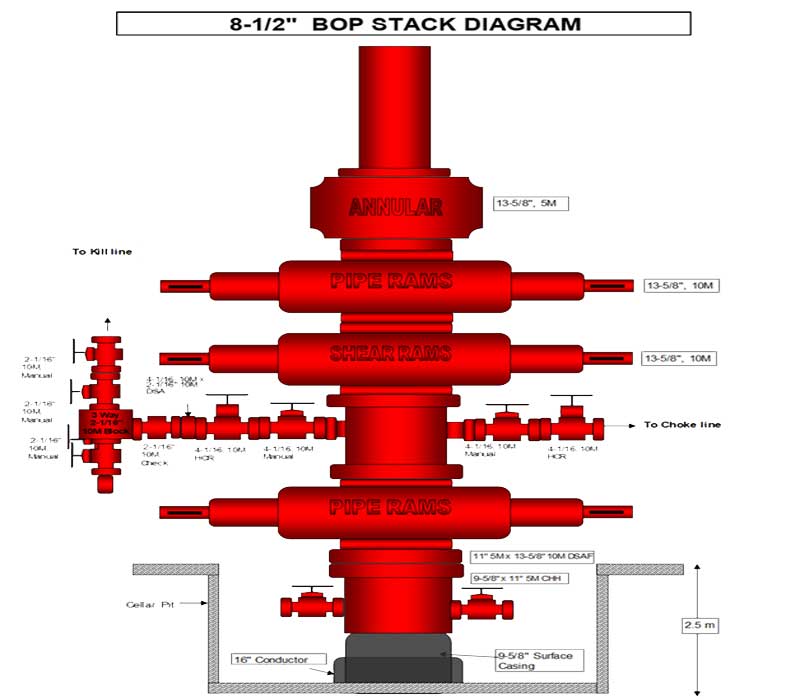
Killing a well or controlling a kick is stopping a well from flowing or having the ability to stop formation
Read More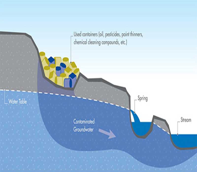
The potential for pollution entering your well is affected by its placement and construction — how close is your well
Read More