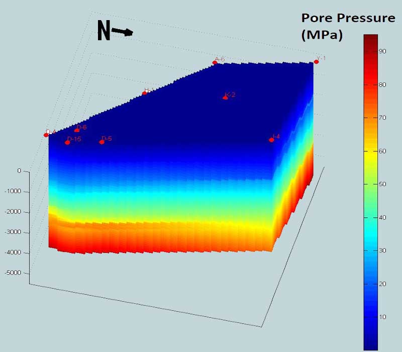
Quantitative Methods of Real-Time Pore Pressure and Wellbore Stability Detection

Our pore pressure computer program (Geopressure software)  for detection / analysis of abnormal pore pressures during mud logging (drilling) operation currently supports the following methods:

Overburden gradient calculation

Formation Pressure calculation by:

• Equivalent Depth Method
• Ratios Method
• Eaton Method

Fracture Gradient Calculation by:

• Eaton Method
• Daines Method

Shear failure gradient (SFG) or borehole collapse pressure gradient calculation by:

• Mohr-Coulomb failure criterion

Normal compaction trend line (NCTL) Methods

These are the most common methods in current use, and require a shale sensitive log, a porosity-sensitive log, and an overburden gradient curve corrected for water depth.

• Compute overburden gradient and correct for water depth
• Identify the shale points. Select porosity points at the shale points.
• Determine the normally compacted interval in the porosity-sensitive log and fit it with a normal compaction trend line (NCTL)

Compare each point of the porosity log to the NCTL and compute abnormal formation pressure using an appropriate method.

In practice, fracture gradient also is calculated and plotted with the pressure/overburden curves.

Estimating Overburden Gradient

• For evaluation of formation pressure
• For calculation of fracture gradient

The Operator can hand-calculate an approximate overburden curve from formation bulk densities for several representative depths over the interval to be drilled. Representative bulk densities may derive from wireline log data, from ‘shale’ (cuttings) densities, or seismic (interval velocity) data.

If we have an electric log for the formation density, we can use it to calculate the overburden:

Divide the log into intervals of depth with similar density.

If the proposed well is offshore, the first two density intervals will be:

• Air gap between elevation of flowline and mean sea level, with ρb= density of air

• Water depth between mean sea level and sea bottom (mud line), with ρb = density of sea water.

Then fill the following form to calculate the overburden at the end of each depth interval:

Interval bottom (m)	Thickness (m)	Bulk density (kg/)	Overburden pressure in the interval (kg/cm2)	Total overburden pressure (kg/cm2)	Overburden gradient (kg/cm2/10m)
150	150	1.06	S=150*1.06/10 = 15.9	15.9	GS= 15.9*10/150 = 1.06
400	250	1.70	S=250*1.70/10 = 42.5	15.9 + 42.5 = 58.4	GS= 58.4*10/400 = 1.46
700	300	1.80	54.0	112.4	1.61
1070	370	1.89	69.9	182.3	1.70

Plotting the overburden gradient versus depth gives a curve

The equation of the curve is:

S= a(Ln(Depth))2+ bLn(depth) + c

The coefficients a, b and c are regional characteristics

If no density log is available,

a ”hard formation” or a “soft formation” set of coefficients a-b-c is used.

The default coefficients, known as ‘soft’ and ‘hard’ values, were constructed from data for a number of wells in two separate areas:

‘Soft’ coefficients (relatively pure shales)

a = 0.01304

b = -0.17314

c = 1.4335

‘Hard’ coefficients (siliceous shales)

a = 0.01447

b = -0.1835

c = 1.4856

Clients most often prefer to use sonic log densities, or seismic transit times, to calculate formation bulk densities. This set of calculations is known as the AGIP method (Belotti, et al., 1978).

The transit times of sound waves passing through a given formation can be used to define the porosity of the rock, as in the equation below:

Where:

⧍t_log = Transit time reading from the sonic log (μsec/ft)

⧍t_m = Rock matrix transit time (μsec/ft)

⧍t_f = Transit time of the formation fluid (μsec/ft)

∅ = Porosity (decimal value from 0 to 1)

In practice, the approximate value of ⧍t_f is 200 μsec/ft. The values for ⧍t_m can be approximated as below

Lithology	Density (kg/l)	⧍tma (μsec/ft)
Dolomite	2.87	43.5
Limestone	2.71	43.5 to 47.6
Sandstone	2.65	47.6 to 55.6
Anhydrite	2.96	50
Salt	2.02	67
Shale	3*	47*

Three formulae describe the relationship between porosity and transit times for different types of sedimentary formations.

After approximating the porosity, the bulk density is a function of:

Where:

ρb = Bulk density for the interval, g/cc

ρm = Rock matrix density, g/cc

ρf = Formation fluid density (usually 1.03), g/cc

Requirements for formation pressure/fracture gradient FP/Frac Calculations

For estimated formation pressure calculations, you will need:

• DCN (‘normal’ trend of compaction increase)
• Overburden gradient
• Normal formation pressure (mud density equivalent) or equilibrium density at a specific depth.

For fracture gradient calculations, you will need:

• Effective vertical stress
• Tectonic stress (if Daines Method is used)
• Formation pressure gradient.

Estimating formation pressure Pf

Our Pore Pressure Engineers can calculate formation fluid pressures from any of the following data:

• Seismic interval velocities
• Normalized drilling parameters (‘d’ Exponent)
• Shale density
• Wireline or MWD logs, including resistivity/conductivity, sonic and direct measurement of downhole pressure
• RFT/DST (providing direct measurement of pressures)
• Kick.

In practice, ‘d’ Exponent usually provides the primary pressure data, with the other processes used to verify or correlate the results.

Equivalent Depth Method

We can apply the Terzaghi equation for Overburden pressure, (S= σ+ Pf) . We know that we have the same compaction in A and B, so the stress S must be the same in both points! σA = σB

We can write:

σB =  SB – PfB and σA = SA – PfA

As σA = σB  we have:

SB –PfB = SA –PfA

Thus:

PfA = PfB + (SA -SB)

Overpressure applies the equivalent depth method via the following equation:

  DeqA=Sa –  Hb/Ha * (Sb – DeqB)

                           

Where:

DeqA = Equilibrium density at depth A

Sa= Overburden gradient at depth A

Ha= Depth A

DeqB= Equilibrium density at depth B

Sb= Overburden gradient at depth B

Hb= Depth B

Ratios Method

Application:’d’ Exponent, shale density, wireline/MWD logs(resistivty and sonic log)

Principle:

The difference between observed and ‘normal’ values of a parameter is proportional to the increase in pressure.

As an example, for ‘d’ Exponent, the calculation is:

where:

PF = Formation pressure gradient (mud density equivalent)

H= ‘Normal’ pressure gradient (mud density equivalent)

Eaton Method

Application: Interval velocities, ‘d’ Exponent, wireline/MWD logs(resistivty and sonic log)

The Eaton Method uses the principle that changes in the overburden gradient govern the ratio between the observed and ‘normal’ values of a given parameter.

Shale Resistivity:

Pf Gradient=OVBG – (OVBG – H)*(Rsh_{O /} Rsh_N)^1.2

                                                                    

With H:  normal hydrostatic gradient

         Rsh_N: Theorical shale resistivity on normal trend (B)

          Rsh_O: Observed value of shale resistivity         (A)

         OVBG: Overburden gradient observed at observed depth

Sonic:

Pf Gradient=OVBG–  (OVBG – H)*( Dt_N /Dt_O)^3.0

                                                                                 

With H:  normal hydrostatic gradient

         Dt_N : Theorical transit time on normal trend (B)

          Dt_O : Observed value of transit time     (A)

        OVBG: Overburden gradient observed at observed depth

Formation tests

DST or RFT tests give a direct evaluation of the Pf

Estimating Formation Pressure from Kick

In most kicks, the invading fluid does not enter the drill pipe. Thus, the Shut-in Drill Pipe Pressure (SIDPP) represents the amount by which formation pressure exceeds the hydrostatic pressure of the mud column.

Formation pressure equals the sum of mud hydrostatic pressure (inside the drill pipe) plus Shut-in Drill Pipe Pressure (SIDPP).

Calculating Fracture Gradient

Liquid exerts pressure which is equal in all directions.

When solids are subjected to external force, it reacts by distributing internal load called stress -giving to stress ellipsoid.

If loading is perpendicular to eliminatory surface the stress is normal.

If loading is tangential to the eliminatory surface shear stress results.

σ = OVB – PF

Fracture occurs when the stress exceeds tensile strength of the rock.

The pressure in this case is fracture initiating pressure. – FP1

If the pressure is suddenly reduced the fracture closes.

To reopen the existing fracture less pressure required – FP2

A surge may open a fracture, afterwards the mud that was holding the hole may not hold any more. Stress is a pressure force per unit area and acts normal to the selected plane.

Stresses acting at any point can be resolved in to 3 mutually perpendicular stresses.

Maximum – σ1

Intermediate – σ2

Minimum – σ3

Relaxed area : Low topography σ1 is vertical and equal to the weight of the overlying rocks.

σ2 and σ3 are horizontal and normal to σ1 .    σ1 > σ2 = σ3

Extreme case:

Tectonically stressed area : Thrust faults etc. σ3 is vertical and equal to weight of overlying rocks.

σ1 and σ2 are horizontal.

When fracture occurs S3 is overcome.

Fracture Pressure  F = S3= σ3 + PF                 σ3 = K X σ1

F – PF = K X σ1

          K  X (OVB – PF)

( F – PF) / (OVB -PF) = K (Stress Ratio).

Thus K can be calculated after LOT. Values of K differ with depth.

Hence a plot of Depth X K is necessary to get proper value of fracture pressure.

Poisson’s Ratio

Eaton introduced Poisson’s ratio to account for variable overburden gradient.

The ratio of lateral unit strain to the longitudinal strain in a body that has been stressed longitudinally within its elastic limits.

Measure an ability of the rock to deform within its limits.

Fracture Pressure F = [ μ/ ( 1- μ)] σ1+ PF

Consider flat lying stratum of semi-infinite extent and weight of overlying strata is the only source of stress.

σ H = [ μ / ( 1- μ)] σ1         μ = 0.25

= [ 0.25  / ( 1 – 0.25) ] σ1

= 1 / 3 (σ1 )

Calculating Frac: Eaton Method

As described previously, Eaton uses Leak-off Test results to compute Poisson’s ratio; this ratio is then use to determine the corresponding fracture gradient:

The fracture gradient at a specific depth is then calculated as a function of:

Calculating Frac: Daines Method

The Daines Method refines the Eaton calculation by allowing for a variable Poisson coefficient based on rock type drilled, and by introducing a correction factor for tectonic stress.

The basic Daines calculation is:

Frac = σ_{t +} σ (μ)/(1 – μ) +    PF ; where σ is vertical effective stress

Data from the first Leak-Off test (in a compacted formation) allows back-calculation of the ratio of superimposed tectonic stress:

σ_t = Frac –  σ ( (μ  )/(1 – μ)+    PF )

To determine the tectonic stress at the Leak-off Test depth:

σt = Frac- σ’1  X  μ/1 – μ+    P

Where:

σt = tectonic stress

Frac = Formation fracture gradient (mud weight equivalent); determined from leak-off test pressure

σ’1 = maximum effective compressive stress

μ = Poisson’s Ratio, as determined from table on next slide

P = estimated formation pressure gradient (mud weight equivalent).

Daines suggested the following Poisson’s ratios for different lithologies (use the one that most closely corresponds to the rock type at the Leak-off Test depth:

Rock type	μ	Rock Type	μ
Clay	0.17 to 0.50	Sandstone cont.
Conglomerate	0.20	poorly sorted, shaly	0.24
Dolomite	0.21	fossiliferous	0.01
Limestone:		Shale:
micritic	0.28	calcareous	0.14
sparitic	0.31	dolomitic	0.28
porous	0.20	siliceous	0.12
fossiliferous	0.09	silty	0.17
argillaceous 0.17	0.17	sandy	0.12
Sandstone:		kerogenaceous	0.25
coarse	0.05 to 0.10	Siltstone	0.08
medium	0.06	Slate	0.13
fine	0.03	Tuff, glassy	0.34

After Daines, Journal of Petroleum Technology, 1982

The maximum effective compressive stress is determined as follows:

σ’1 = S – P

Where:

S = overburden gradient

P = estimated formation pressure gradient (mud weight equivalent).

Indicators from Wellbore Instability

When the mud weight is inappropriate, wellbore instability events occur while drilling, which can help to diagnose the overpressure and to adjust mud weight in real-time drilling operations. Wellbore instability can be classified into two categories:

• Shear failures
• Tensile failures.

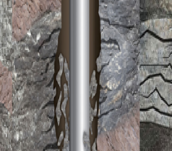
Shear failures

When the downhole mud weight is less than the shear failure gradient (SFG, or borehole collapse pressure gradient), the wellbore experiences shear failure.  Shear failure is mainly caused by the condition in which the applied mud weight is lower than the SFG. The indicators of shear failures while drilling include hole enlargement (borehole breakout), hole closure, tight hole (overpull), high toque, hole fill after trip, hole bridging, hole pack-off, and hole collapse.

 Some of these indicators may be caused by swelling shale when the water-based mud is used because of the chemical reaction between the mud and the shale formation. Therefore, it needs to identify the causes of the failures.

Here we use a vertical well as an example to illustrate the relationship of wellbore instability and pore pressure. Based on Mohr-Coulomb failure criterion, the minimum mud weight to avoid borehole shear failure can be obtained from the following equation:

P_m  = 1 – sin φ/2 (3σ_{H –} σ _{h – UCS}) + p_{p sinφ}   

Where 

P_m  = minimum mud pressure or collapse (shear failure) pressure

 _φ = angle of friction of the rock

 UCS = rock uniaxial compressive strength

p_{p =} Pore pressure

σ_H, σ _h = the maximum and minimum horizontal stresses, respectively.

The horizontal stresses are most important parameters for analyzing wellbore stability, which can be obtained from either field measurements or calculations

The equation above shows that the shear failure is directly related to the pore pressure; a higher pore pressure needs a heavier mud weight to keep the wellbore from the shear failure. Therefore, wellbore instability can be used as an indicator of an overpressured formation.

Tensile failure

Tensile failure occurs when the mud pressure exceeds the capacity of the near-wellbore rock to bear tensile stress. If the downhole mud weight is higher than the fracture gradient, the formation will be fractured to create hydraulic fractures (or drilling-induced tensile fractures). Real-time indicators of drilling-induced tensile failures include hole ballooning, drilling mud losses, and lost circulation. Reducing mud weight, adding lost circulation materials (LCM), or applying wellbore strengthening technique are possible cures for the drilling-induced tensile failures.

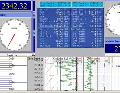
Procedures of Real-Time Pore Pressure Detection

For real-time pore pressure detection and monitoring, the following steps can be performed:

• Construct predrill petrophysical and pore pressure model and calibrate the predrill model to offset wells if they are available. The model includes methods of resistivity, sonic, Dxc, and so on. The model should include uncertainties and address drilling challenges and potential issues.

• Apply the model to the real-time well. It particularly needs to have a calibrated NCT for each method.

• Connect the model to real-time data (e.g., use Connect WITSML to connect LWD and MWD tools), so that the real-time data can be automatically loaded to the model. The model can then automatically calculate pore pressures based on the NCT using the real-time LWD and MWD data.

• Compare the real-time calculated pore pressure to downhole mud weight (ESD, ECD); to determine if the mud weight is sufficient, particularly it needs to identify whether or not the mud weight is less than the pore pressure gradient. Only comparing the real-time calculated pore pressure gradient to the mud weight is not enough to conclude an underbalanced drilling status. Therefore, it also needs to combine to other real-time indicators of pore pressures.

• Adjust the models (mainly NCTs) based on the following data if they are available: real-time pore pressure measurement, well influx, mud pit gains, kicks, mud gas data, mud losses, drilling parameters, and borehole instability events (e.g., cavings, torque, fills, and pack-offs).

• Alert and inform the rig for action when the pore pressure is lower (underbalanced) or close to the downhole mud weight.

• Liaise with technical expert group on all issues related to unplanned drilling operations, ECD, and pore pressures.

• Make postwell knowledge capture and transfer within the appropriate organizations and systems.

                                               

The real-time monitoring should ensure that:

• Pore pressure is continuously monitored and indicators of the abnormal pressures are identified;

• Real-time pore pressure methods, estimates, and updates are discussed routinely with all involved monitoring parties to provide a consistent interpretation to the rig operations;

• Abnormal pore pressure events are identified as soon as possible;

• The abnormal events, including significant observations, changes, or updates in pore pressure estimates, if they are occurring or imminent, need to be communicated to the operations (e.g., operation geologist and drilling engineer) quickly;

• The appropriate actions of operations (e.g. raising mud weight when the pore pressure gradient is lower than the downhole mud weight) are taken quickly.

Talk to us for your upcoming Pore-Pressure and Wellbore-Stability Prediction requirement

Geodata Evaluation & Drilling LTD. Pore pressure consultant use specialist software to provide pore pressure profiles for your wells which are calibrated to offset well behavior for determination of optimum mud weight window for successful drilling operation. Contact us at www.geodatadrilling.com Phone: +234 8037055441