Borehole drilling, Soil investigation, Geophysical, Environmental, Oil and Gas

Category: Oil and Gas Services (Page 1 of 2)

How to Perform Secondary Well Control While Drilling

Secondary Well Control

If due to any reason hydrostatic pressure in the well bore falls below the formation pressure, formation fluid may enter in the well bore (Kick) and if so happens, the primary control may be temporarily lost and a proper use of blowout preventers and kill procedures will provide Secondary well control, or in other words secondary well control involves detection & safe handling of kicks so as to re-establish primary well control.

Positive Kick Signs

In addition to kick warning signs that was discussed previous in the post on how to carry out primary well control: https://geodatadrilling.com/blog/2023/01/05/how-to-carryout-primary-well-control-while-drilling/ A Positive kick indicators are different from kick warning signs. They indicate that the kick has already entered the well bore. For any of the following positive kick sign, a flow check is required.

Increase in return flow (Pumps On)

After the early warning signs, the first positive kick sign is increase in flow rate at the flow line with pumps on. The entrance of any fluid into the well bore causes the flow rate to increase.

Flow from well (Pumps Off)

Stopping the pump causes a reduction in bottom hole pressure equivalent to the annular pressure drops, so flow check is a reliable method of checking for a well kick. If the well does not flow when the pump is shut off and remains static for two or three minutes, then no well kick is entering.

Pit Volume Increase

An increase in pit volume is obvious & positive indication of flow into the well bore & can be easily verified. If an increase in pit volume is seen, shut off the pump and make a flow check. If the well does not flow, no kick is entering.

Decrease in Pump Pressure and Increase in Pump Stroke

In case of kick there is under balanced condition between the fluid in the drill pipe and the mixed column of mud and influx in the annulus. Therefore, circulating pressure gradually decreases and unless the pump throttle is changed, pump speed slowly increases.

When one or more positive kick signs are observed, flow check is made. In case of self-flow, well can be shut-in. Blow Out Preventer is an equipment use to shut-in well and provide secondary well control.

Surface Well Control Equipment – BOP

Fig 1. 8.5” BOP STACK

Annular

Consist of a single doughnut shaped element which, when pressurized by hydraulic fluid, will close on any object in the well. Most annulars are ‘well bore pressure assisted’ in that the force up helps the packing element to close in the well. The energy to close the rig BOPs is hydraulic fluid supplied via an accumulator system. If this hydraulic system fails, annulars will have a tendency to open unless check valves are placed in the closing line. Annulars are not designed to hold pressure from above.

Pipe Rams

Consist of two specifically sized elements which will close on the body of a specific size of tubular but not its connections – a derivative of this is a variable bore pipe ram (VBR) which are used to close around tubulars of different sizes within a limited range.

Pipe rams are not designed to hold pressure from above – subsea pipe rams particularly are designed to support the weight of a drill string. They are designed to stay closed if hydraulic power is lost from the line to the closing chamber and will automatically open when the opening chamber is activated, or in the case of one type can be locked and unlocked separately. Surface pipe rams can be closed manually.

The normal operating pressure of ram preventers is 1500 psi. 3000 psi can be applied by utilizing a bypass valve on the hydraulic accumulator unit on the surface unit. A separate circuit is used subsea for 3000 psi closing pressure for shear rams.

The main components of ram preventers are:

  • Ram assembly including seals, and ram
  • Ram shaft
  • Bonnet
  • Piston
  • Operating cylinder
  • Side outlets

Blind Shear Ram

Blind Shear Ram will close and seal on open hole and cut tubular in the well or, if no tubular is present, it will seal on open hole. Blind rams without the shear facility will not cut pipe. It is good practice to test blind/shear rams with the range of pipe likely to be used in the well, clearly the shearing blades in most cases will have to be replaced if used in anger or after testing their cutting capability.

Safety Valves – Kick While Tripping

If the well kicks whilst tripping then a safety valve will have to be stabbed to secure the drill stem first before closing a blow-out preventer (BOP). These are sometimes called inside BOPs (IBOPs). Both valves need crossovers for the particular size of tubing and a quick and efficient way of stabbing the valve safely.

Fig 2. Safety Valves

Surface Hook-up of Well Control Equipment

A typical surface hook up is shown in Figure 3. The choke manifold is a high-pressure routing device rated to the same working pressure as the stack. It should have at least two variable valves called chokes, one manual and one remote hydraulic, controlled from a choke panel positioned on the rig floor.

Fig 3. BOP and Choke Manifold Arrangement

Valves on the kill line side, at the left of the spool, are closed during normal operations. The one on the right side of the spool is open during normal operations. The HCR (High Closing Ratio) valve is opened and closed remotely from the BOP panel at the rig floor. Fig 3 is a panel showing the schematic of the stack and all BOPs can be closed from the BOP panel or directly from the accumulator-closing unit.

Shut in procedures – Surface stack

In all cases, when the pumps are being used, eg. drilling ahead, the pump(s) are kept running until just before the BOP is closed. This enables the annulus pressure loss (APL) element of the circulating pressure to aid the BHP against the formation pressure and should help minimise the kick size. It is imperative that the well is closed in with the least gain (kick size) – particularly when the kick fluid is gas which will give the largest annulus pressures compared to a liquid kick – when circulating the kick fluid out of the well

Fig 4. Circuit Alignment in Hard Shut in Procedure

Hard Shut-in – Surface Stack

  1.  Pick-ups off bottom until first tool joint above rotary table (Kelly).
  2. Switch off pump(s).
  3. Close BOP.
  4. Open HCR to read annulus pressure and read drill pipe pressure. (This procedure according to API RP59 – therefore either annular or ram can be closed – if ram then tool joint must be clear off pipe ram.)
  5. Note kick size (pit gain).

Fast Shut-in – Surface Stack

  1. Pick up off bottom as hard shut in.
  2. Switch off pump(s).
  3. Open HCR valve.
  4. Close annular BOP.
  5. Read drill pipe and annulus pressure and record pit gain.

In both hard and fast shut-in methods the chokes are closed as part of the pre-kick choke manifold line up.

Soft Shut-in

The pre-kick choke manifold line up for the soft shut in includes all lines open to the mud/gas separator – this includes the designated choke which is also open.

The only valve isolating the circulating system from the mud/gas separator is the HCR.

  1. Pick up off bottom until first tool joint above rotary (if Kelly).
  2. Switch off pumps.
  3. Open HCR.
  4. Close annular BOP.
  5. Close choke.
  6. Read drill pipe and annulus pressure and note kick size (pit gain).

Companies will choose which shut in procedure to use for their operations. However, the evidence to suggest hydraulic shock by shutting the well in too quickly is not evident. This is the reason given for the so-called soft shut in. It means more gain – which is undesirable.

The hard shut-in is the quickest method of shutting in the well but the HCR is not opened until the well is shut-in. This could put a shock into the choke line if the annulus pressure is excessive. Not so excessive for surface stacks with relatively short choke lines, but not advisable for subsea stacks with longer choke lines.

The fast shut in is probably the least contentious, with potentially less gains than the soft shut more gain compared with the hard shut-in, but less shock to choke line than hard shut- in.

In nearly every case, the valve behind the choke is closed when the well is shut-in, this adds extra security and ensures no further influx if the variable choke is leaking.

Clearly the soft or hard shut-in could be used but, as explained earlier, the fast shut-in has fewer chokes line shock than hard shut-in and less kick volume than soft shut-in.

How to Carryout Primary Well Control While Drilling

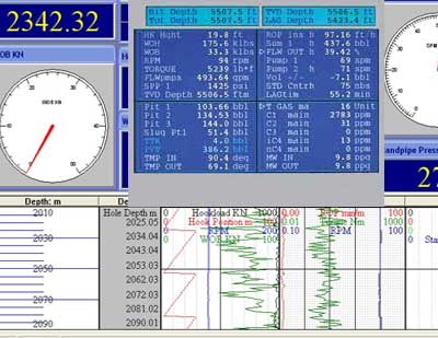
Definition of Primary Well Control:

This is the name given to the process that maintains hydrostatic pressure in a well bore greater than the formation fluid pressure but less than fracture pressure.

If hydrostatic pressure is less than formation pressure then unwanted formation fluids will enter the well bore. If the hydrostatic pressure of the fluid in the well bore exceeds the fracture pressure of the formation then the hydrostatic pressure of the fluid in the well bore will decrease possibly to a point where formation pressure will exceed hydrostatic pressure and formation fluids will enter the well bore. An overbalance of hydrostatic over formation pressure is maintained – this is normally referred to as a trip margin.

Secondary Well Control

If the hydrostatic pressure of the fluid in the well bore fails to prevent formation fluids entering the well bore the well will flow uncontrollably until all pressure is dissipated. This process is stopped using a blow-out preventer to prevent the well bore fluids escaping from the well – this is the initial stage of secondary well control – containment of unwanted formation fluids.

For the purpose of this guidance note, we are going to focus on primary well control. However, secondary well control will be discussed in a separate post.

As previously stated Primary Well Control is a process that maintains hydrostatic pressure in a well bore greater than the formation fluid pressure but less than fracture pressure to prevent unwanted fluid entering the wellbore.

What is Hydrostatic, Fracture Pressure and Formation Fluid Pressure?

Hydrostatic Pressure:

The pressure exerted by a column of fluid depends on its density and vertical height or depth. Hydrostatic Pressure (psi) =Mud weight (ppg) x 0.052 (psi/ft) x True Vertical Depth (TVD)ft

Where:    

psi  = pounds per square inch.

ppg   = pounds per gallon.

0.052     = pounds per square inch per vertical foot of a 1 pound per gallon fluid.

Since pressure is measured in Ibs per square inch (psi) and depth is measured in feet, it is convenient to convert mud weight from Ibs per gallon (ppg) to a pressure gradient in psi/ft.

The 0.052 conversion factor is derived as follows: 1 cubic ft. contains 7.48 US gallons. A fluid weighing 1ppg would weigh 7.48Ibs per cubic ft.

The pressure exerted by that one ft. height of fluid over the area of the base would be:

7.48 pounds/144 square inches = 0.0519 pounds per square inch (psi) Hence, a one ft. high column of 1ppg fluid would exert 0.052 psi on its base. This is the same as saying the pressure gradient of the fluid is 0.052 psi/ft.

ppg x 0.052 ( mud weight)    =          psi/ft. (pressure gradient)

Formation Fracture Pressure

Formation fracture pressure, or formation breakdown pressure is the pressure required to rupture a formation, so that whole mud can flow into it. The symbol PFB is usually used to denote this pressure.

Commonly this is expressed as a pressure gradient, GFB, with the units of psi/ft.

The formation breakdown pressure is usually determined for formations just below a casing shoe by means of a leak-off test (LOT). This test of the formation strength, also known as a formation integrity test or FIT, is effected after the casing has been run and cemented in place. This allows formations to be tested after the minimum of disturbance and damage due to drilling, and allows a clear indication of strength to be determined for one isolated zone.

Leak Off Test (LOT) Procedures and Calculations

  1. Drill out new formation few feet, circulate bottom up and collect sample to confirm that new formation is drilled to and then pull string into the casing.
  2. Close annular preventer or pipe rams, line up a pump, normally a cement pump, and circulate through an open choke line to ensure that surface line is fully filled with drilling fluid.
  3. Stop the pump and close a choke valve.
  4. Gradually pump small amount of drilling fluid into well with constant pump stroke. Record total pump strokes, drill pipe pressure and casing pressure. Drill pipe pressure and casing pressure will be increased continually while pumping mud in hole. When plot a graph between strokes pumped and pressure, if formation is not broken, a graph will demonstrate straight line relationship. When pressure exceeds formation strength, formation will be broken and let drilling fluid permeate into formation, therefore a trend of drill pipe/casing pressure will deviate from straight line that mean formation is broken and is injected by drilling fluid. We may call pressure when deviated from straight line as leak off test pressure.
  5. Bleed off pressure and open up the well. Then proceed drilling operation.


Oilfield Unit

Leak Off Test pressure in mud density

Leak off test in equivalent mud weight = (Leak Off Test pressure ÷ 0.052 ÷ Casing Shoe TVD) + (Current Mud Weight)

Where;

Leak off test in equivalent mud weight in ppg

Leak Off Test pressure in psi

Casing Shoe TVD in ft

Current Mud Weight in ppg

Note: Always round down for LOT calculation

Example:

Leak off test pressure = 1,600 psi

Casing shoe TVD = 4,000 ft

Mud weight = 9.2 ppg

Leak off test in equivalent mud weight (ppg) = (1,600 psi ÷ 0.052 ÷ 4,000 ft) + 9.2ppg = 16.8 ppg

Leak Off Test Graph

Formation Integrity Test (FIT) Procedure and Calculation

Formation Integrity Test is a method to test strength of formation and casing shoe by increasing Bottom Hole Pressure (BHP) to designed pressure. FIT is normally conducted to ensure that formation below a casing shoe will not be broken while drilling the next section with higher BHP or circulating gas influx in a well control situation. Normally, drilling engineers will design how much formation integrity test pressure required for each hole section.

The formula below demonstrates how to calculate required FIT pressure.

Pressure required for FIT = (Required FIT – Current Mud Weight) × 0.052 × True Vertical Depth of shoe

Where:

Pressure required for FIT in psi

Required FIT in ppg

Current Mud Weight in ppg

True Vertical Depth of shoe in ft

Note: FIT pressure must be rounded down.

Example:

Required FIT (ppg) = 14.5

Current mud weight (ppg) = 9.2

Shoe depth TVD (ft) = 4000 TVD

Pressure required for FIT = (14.5-9.2) × 0.052 × 4000 = 1,102 psi

Maximum Allowable Annular Surface Pressure

The leak-off pressure, PLO, is determined as the maximum surface pressure, which the well could stand, with the hydrostatic load of mud in use at the time of the test. This can be described as the Maximum Allowable Annular Surface Pressure (MAASP) with that particular mud weight in use (meantime we shall leave aside safety factors).

Every time the mud weight is changed, the MAASP changes and must be recalculated.

MAASP = (GFB – CMUD) x Shoe Depth, True Vertical

If a Maximum Equivalent Mud WT is quoted for formation strength, then the same formula appears as:

MAASP = (Max Equiv. Mud Wt(ppg) – Current Mud Wt(ppg) x 0.052 x Shoe Depth, True Vertical

Frequently a safety factor is applied so that the ‘actual’ maximum is never applied.

This safety factor gives a margin for error. A leak-off test is not usually a precise or high accuracy test, so a margin, and a value somewhat lower than the formation fracture is used, particularly when the ECD is a major factor.

Formation Fluid Pressure (PF)

The formation fluid pressure, or pore pressure, is the pressure exerted by the fluids within the formations being drilled.

The sedimentary rocks, which are of primary importance in the search for, and development of oil fields, contain fluid due to their mode of formation.

Most sedimentary rocks are formed as accumulation of rock debris or organic material, underwater. Since over two thirds of the earth’s surface is covered with oceans, the vast majority of sedimentary rocks are laid down as marine sediments in the shallow seas around the land areas.

In general, areas of the earth’s surface, which are above sea level, are affected by the processes of erosion (breaking up and wearing down of the land masses). The debris is washed down into the shallow sea basins where it settles out onto the sea floor, the coarser material generally settling out closer to the shore than the fine silts and clays.

This process may continue for long periods as the earth’s surface slowly moves, some areas being pushed up to provide fresh surfaces for erosion, with adjacent sea basins slowly deepening to allow great lengths of sediment to build up. Thus sedimentary rocks contain water, usually seawater, as an integral part of their make-up. As the depth of sediment increases, the rocks are compacted, squeezing water out. The water contained within the rocks becomes progressively more salty as the relatively small molecules of water move through the pore spaces of the rock, while the larger salt molecule is retained.

The result of this is that the formation fluid pressure, or pore pressure, exerted by the water in a normal, open, sedimentary sequence is equivalent to that produced by a free-standing column of salt water, which is rather saltier and heavier than typical sea water.

An average figure for normal formation pressure gradient in marine basin sediment determined some years ago in the US Gulf Coast area is 0.465 psi/ft. This is the pressure gradient produced by a column of water of approximately 100,000 ppm chloride. In comparison, a typical value for seawater is 23,000 pprn chloride.

This gradient of 0.465 psi/ft. or expressed as an equivalent mud weight, 8.94 ppg is generally accepted as a representative figure for normal pore pressures in marine basins in the Gulf of Mexico. a common value for the North Sea is 0.452 psi/ft.

Abnormal Pressures

Abnormal formation fluid pressure, or ‘sur-pressures’ as they are sometimes known, are pressures greater than normal formation pressure and can rise for a number of reasons. They can be categorized as:

  • Under compaction
  • Artesian Effect
  • Faulting
  • Salt Dome
  • Gas Cap Effect
  • Charged Sand

The above causes of Abnormal Pressure will be discussed in another post

As discussed previously, Primary Well Control is a process that maintains hydrostatic pressure in a well bore greater than the formation fluid pressure but less than fracture pressure to prevent influx of formation fluid to the wellbore.

Definition of Influx and Kick

An influx is an intrusion of unwanted formation fluids into the well bore which does not immediately cause formation pressure to exceed the hydrostatic pressure of the fluid in the well bore – but may do if not immediately recognized as an influx – particularly if the formation fluid is gas. A kick is an intrusion of unwanted fluids into the well bore such that the formation fluid pressure exceeds the effective hydrostatic pressure of the well bore fluid.

There are some warning signs to watch out for while drilling to ensure drilling mud weight (hydrostatic pressure of the well) is adjusted to mitigate formation fluid influx to the wellbore.

Kick or Influx Warning Signs

DURING TRIPPING

The indication of the presence of a kick or influx is:

  • Incorrect hold fill volume

If this sign is not noticed at an early stage, it should become progressively more obvious. In the more extreme case the hole would eventually stay full, or flow, while pulling out.

  • Hole keeps flowing between stands, while running in

The presence of some or all of these indications requires that a flow check is carried out to determine whether or not a kick is in progress.

DURING OR AFTER TRIPPING

Trip gas is a measure of swabbed gas over an entire trip. Often a short trip of 15-20 stands is made in order to circulate bottoms up and measure units of swabbed gas. Excessive units of trip gas may indicate the need for increasing the trip margin and/or reducing swab pressure.

DURING DRILLING

The general definition of a warning sign – particularly while drilling is:

‘It is a sign to indicate a kick or some other reason’

However, vigilance and care are exercised to ensure that the reason for the sign is investigated.

The following warning signs are given in approximate order of priority. The drilling break is considered the most important and must always be investigated.

Drilling Break

A sudden increase in rate of penetration is usually caused by a change in formation type. It may however signal an increase in permeability and an increase in formation pressure. Both these effects result in faster drilling.

The drilling break may be dramatic, though most commonly a gradual change is seen. A drilling break could indicate a kick is in progress though it is often a sign that conditions are changing and formation pressure rising, which may lead to a kick.

Gas-Cut Mud

The appearance of gas cut mud at the surface usually causes concern, particularly bottoms up after a connections The reduction of bottom hole pressure owning to gas cutting can be critical on surface hole. However, due to the compressibility of gas, a fifty percent gas cut of mud at the surface changes the bottom hole pressure at 20,000 feet may be only 100 psi. The relative decrease in surface hole would be critical and the gas must be eradicated.

Gas cutting must not be ignored and the cause must be investigated.

Pump Pressure Decrease/Pump Stroke increase

Invading formation fluid generally reduces the total head of fluid in the annulus. The head of mud in the drill pipe is unaffected, so that there is a tendency for fluid to ‘U- tube’. This means that the pump does not have to provide so much energy and this may be seen as a pump pressured reduction. Depending on the rig installation, a small increase in pump rate may also be noted.

The effect is small, and may not be noticeable. The same effects are seen if a washout occurs, so it is necessary to confirm which is taken place, by doing a flow check. The presence of a continuous recording rnonitor of pump pressure and pump stroke rate on the drill floor means that quite small changes can be seen readily by the Driller.

Total Gas Levels

A gas detector, or hot wire device, provides valuable information. Such instruments measure changes in the relative amounts of gas in the mud and cuttings, but do not provide a quantitative value. Increase in the gas content can mean an increase in gas content of the formation being drilled, gas from cuttings and/ or an underbalanced pressure condition.

In conditions of normal pressure and normal overbalance, background gas should not vary significantly as the hole is drilled. Changes in background levels indicate possible conditions of concern. Increases in the normal background gas indicate the flow of formation gas into the mud or the presence of gas expanding from drilled cuttings. Background gas could mask connection gas, care must be exercised, especially top hole drilling.

Connection gas is a measure of gas which enters the hole whilst making a connections It is reported in units of gas over normal background gas. Estimating the time to pump mud from bottom and checking the gas detector recording can identify connection gas. After the swabbed gas passes the detector, the units should return to the background levels. If not, an underbalance condition could exist.

Connection gas can be eliminated if a sufficiently high overbalance exists, or if pulling speed is reduced and/or if mud properties are adjusted. However, connection gas can be used as an accurate indicator of formation pressure when drilling with close to a balanced pressure. Increasing levels of connection gas are a reliable warning of an underbalanced pressure condition. The relationship of normal gas content readings to the amount of increase can be used as an indicator of the need to increase mud density.

Change in Flow Properties

The presence of formation, such as hydrogen sulphide will effect the chemical and flow properties of mud. Gas and air will ‘froth’ or foam the mud at the surface, lowering the surface density and sometimes increasing the viscosity of the mud.

Formation fluids, particularly salt mater, which can enter the well bore, can also alter the chemical balance of the mud as well as reduce the density. The result can be a drastic change in chemical and flow properties of the mud. For example, salt water in the mud will cause a drop in pH as will hydrogen sulphide with a consequent increase in viscosity and fluid loss.

Sometimes the changing flow properties of a mud system can be a readable warning signal that the well is underbalanced and a kick is imminent.

Torque and Drag, Fill on Connections

Increases in torque and drag often occur when drilling underbalance through some shale intervals. As the result of this fluid in the shale expands, causing cracking, spalling and sloughing of the shales into the well bore. This condition can cause a build-up of cuttings in the annulus, excessive fill on connections and trips, a build-up in torque and drag and eventually stuck pipe. Increases in torque and drag can be a good indicator of abnormal pressure, especially if used with other indicators.

Drilling Exponent

Plots of drilling rate versus depth are often difficult to interpret because of changes in drilling rate variables such as WOB, RPM and mud properties. In 1986, Jorden and Shirley developed a normalized rate of penetration equation from data gathered on the Gulf Coast. In their relationship, normalized drilling rate was defined as a function of measured drilling rate, bit weight and size and rotary speed in the equation shown below:

The authors provided correlation of field measured pressure data and ‘d’ exponent calculation. They showed that formation pressure could be estimated by first plotting ‘d’ values in shale versus depth, on semilog paper, and determining a normal trend line of decreasing value with depth in the normally pressured section. Then, by determining the differences between the extrapolated values of ‘d’ exponent and those calculated from actual data, the correlation was used to estimate the amount of overpressure at any depth.

The method developed with Gulf Coast data has been applied world-wide with moderate success. Since their original work, others have applied a correction for mud weight to obtain a modified drilling exponent. This is applied in much the same way as the ‘d’ exponent and sometimes it is plotted as 100/d versus depth, for direct comparison with plots of interval transit time.

Shale Density/Cuttings

The examination of shale cuttings and/or cores can provide information on formation pressures. Properties of shale such as bulk density, shale type, size, and shape can be related to abnormal pressures.

Several techniques, such as the graduated density column method or the mud balance method, are available to measure the density of shale cuttings recovered at the shaker. Care must be exercised to separate bottom cuttings from upper hole cavings. Also, cuttings must be properly washed and/or scraped to remove the outer layer of mud contaminated sample. Plots of shale bulk density versus depth are made and the normal trend of increasing density versus depth established. Changes from the normal trend can then be related to changes in formation fluid content, and hence formation fluid pressure.

Shale cuttings, which are drilled underbalanced, tend to produce larger than normal cuttings, larger volumes than normal, and shapes that are more angular, sharp and splintery in appearance. These effects are due in part to the fact that fluid trapped within pores of the shale at high pressure expands when exposed to the lower mud hydrostatic pressure. Therefore, drilling rates and hold size increases as shale continues to expand, crack, spall and slough into the well bore, thereby creating larger and different shaped cuttings or cavings. Volume of cuttings increases due to faster penetration rates and increased hole volume caused by sloughing and caving. Close observation of shale on the shaker along with other indicators can provide a basis for determining an underbalanced condition prior to taking a kick.

Heaving Shales

Excessive volumes of shale cuttings on the shaker may be an indication of an underbalanced condition. Shale is usually porous, but has little or no permeability. Fluids in the pores are subjected to formation pressure, but are not able to flow. However, if a differential pressure exists from the formation to the well bore, such as in the case of abnormal pressure, the fluid pressure causes weakening of the walls of the hole and spalling or heaving of shale into the hole. At the surface an increase in volume of shale cuttings is noted. These cuttings are splintery, angular, and generally larger than normal. If these conditions persist, the mud hydrostatic pressure is probably too low and a kick will occur white drilling the next permeable formation.

Shale Type

The type of clay mineral of which shales are largely composed varies slowly with increasing depth and the swelling clays, sometimes known as ‘gumbos’, progressively give way to the non-swelling type. Near the surface the principal clay minerals are calcium and sodium based montmorillonites and illites. With increasing depth of burial these alter slowly – towards the largely potassium based kaolinites.

This change can be determined roughly in a number of ways, as of which the Methylene Blue test for clay absorption lever determination, and Differential Thermal Analysis for structural water content determination are the best known and most widely used.

Flow line Temperature

The temperature gradient in the transition between normal and abnormal pressure zones often increases to about twice the rate of the normal temperature gradient. Increases of the mud temperature at the surface can also indicate the top of an overpressure section. Consideration must be given to circulation times, trip times, connection times, stabiliser temperature after tripping temperature of mud at suction pit, and other factors such is water depth. An increase in flow line temperature when used with other indicators can show the top of an overpressure section with accuracy.

It is important to note this indicator can be partially or totally masked in offshore drilling from floating vessels by the cooling effect of long lengths of riser and substantial air gaps.

Talk to us for your upcoming Mud logging project for monitoring kick Indicators while drilling

Geodata Evaluation & Drilling Limited offers Mud logging services to Oil and Gas industries. Let us handle the project for you. contact us at www.geodatadrilling.com Phone: +234 8037055441

Pore-Pressure and Wellbore Stability analysis to mitigate High cost of unscheduled drilling events

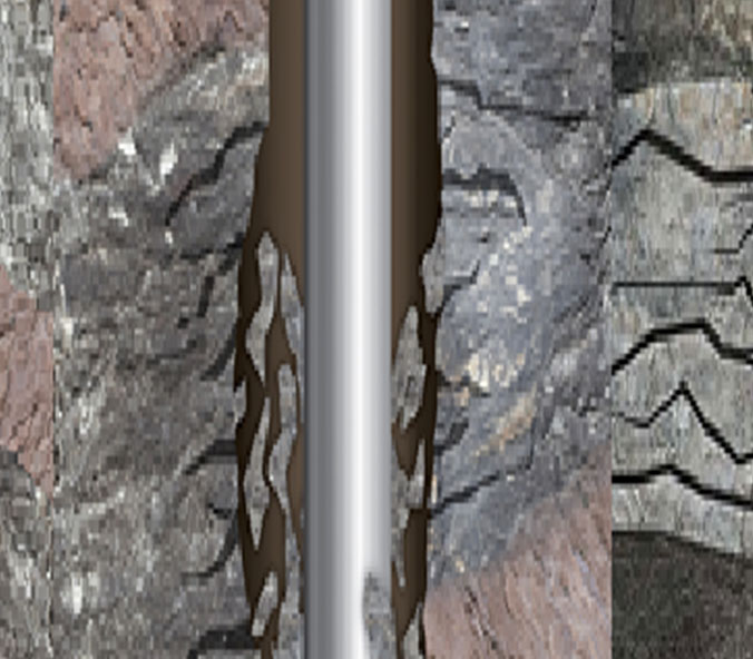
A lack of accurate pore-pressure prediction and wellbore stability analysis can result in unscheduled drilling events, such as blowouts, kicks, hole washouts, wellbore break- out, and stuck pipe. Undetected abnormal pore pressure and wellbore instability also adds to drilling nonproductive time and increase drilling costs in millions of dollars and sometimes leads to abandoning the well before reaching its objective.

Integration of predrill pore-pressure and geomechanics analyses with real-time monitoring consistently provides an effective way to prevent drilling failure and improve well-construction efficiency.

Abnormal pore pressures can cause serious drilling incidents, such as unwanted fluid influx to wellbore (Kick) and well blowouts, if the pressures are not predicted accurately. This can lead to erroneous mud-weight design plan that can contribute to wellbore instability.

A lack of an accurate wellbore-stability prediction can also cause borehole breakouts and in hole closure, pack off, and collapse in cases of tensile and compressive shear failures leading to mud loss and lost circulation through hydraulic fractures and in severe cases can lead to a total lost borehole. Estimated cost to the drilling industry for hole stability problems range from 600 million to 1 billion dollars annually.

Relative cost of unscheduled events caused by wellbore stability problems

When the mud weight, or equivalent circulating density (ECD), is less than the pore pressure, the wellbore experiences splintering failure in shale formation. In this case, wellbore washouts or fluid kicks resulting from underbalanced drilling may occur.

A well may not have fluid kicks in an underbalanced-drilling scenario if impermeable formations that is not over-pressured are penetrated. When the mud weight or ECD is less than the shear-failure gradient or borehole collapse pressure gradient, the wellbore experiences shear failure (or wellbore elliptical enlargement, breakout, or collapse). Wellbore fracturing occurs when mud pressure exceeds the capacity of near-wellbore rock to bear tensile stress and the drilling fluid creates hydraulic fractures.

The drilling-induced fractures may cause drilling-fluid losses and even a total loss of drilling fluid returns (lost circulation). Maintaining wellbore stability and preventing these costly problems require an accurate prediction of the conditions that cause wellbore failures, including pore pressure and safe-mud-weight operating window.

PP=Pore pressure, SFG=Shear failure gradient, FG=Fracture gradient

Pore-pressure prediction

Pore pressure is the fluid pressure in the pore space of the formation. Pore-pressure analyses include three aspects:

  1. Pore pressure analysis before drilling a well include: Seismic data analysis and interpretation in the plan well location; Well-logging, and drilling data in offset wells if available
  2. Pore pressure analysis while drilling a well (qualitative and quantitative): Drilling parameters and mud-logging data; Logging-while-drilling (LWD) or measurement while-drilling (MWD) data
  3. Pore pressure analysis after drilling the well: Wireline log analysis (Sonic log, Resistivity log etc.)

Pore pressure prediction from seismic data analysis before drilling

Bowers (1995) proposed that the seismic interval velocity and effective stress have a power relationship. On the basis of this relationship, pore pressure can be obtained from seismic interval-velocity data (Reflection times to transit times) in the planned-well location. The seismic data transform in terms of depths interval velocities and interval travel times are used for pressure gradient calculation for determination of (Overburden pressure and gradient, Pore pressure and gradient, Fracture pressure and gradient).

Pore pressure gradient from seismic section

Pore pressure prediction from wireline logs and logging while drillings logs

The analysis of wireline logs before drilling for offset wells and logging while drilling (LWD) allows the calculation of:

  • Overburden pressure and gradient
  • Pore pressure and gradient
  • Fracture pressure and gradient

The wireline logs generally used for pressure prediction and evaluation are: Sonic Logs, Induction Logs (Resistivity Logs) and Density Logs.

Pore pressure prediction from LWD data

Pressure prediction and evaluation from drilling and mud-logging data

The acquisition and interpretation of drilling and mudlogging data represent a very important group of techniques which have the advantage to be available more or less in real time while drilling. These methods can be:

  1. Qualitative: Which, if analyzed in their completeness, can provide significant information about the actual status of the well and alert the drilling team of dangerous and abnormal conditions while drilling. Among the qualitative techniques base on drilling and mudlogging data include:
  • Drilling Rate
  • ‘d’ exponent, Sigma log
  • LWD (Resistivity, Density, Sonic)
  • Drag and torque
  • Mud pit level, Return flow, Pump Pressure (kick)
  • After Lag Time: Gas, (BG, CG, Pump off Gas) MW (out), Cuttings Shape/Size, Lithology (anhydrite, known marker, etc.), Shale density, Shale factor, Temp(out)

These are discussed in : “Pore-Pressure and Wellbore-Stability Prediction for Prevention of Drilling incident”.

2. Quantitative: Which ensure the quantification of the pressures acting in and around the well and the related risk levels. These include:

  • Overburden gradient calculation
  • Formation Pressure calculation by:
  • Equivalent Depth Method
  • Ratios Method
  • Eaton Method
  • Fracture Gradient Calculation by:
  • Eaton Method
  • Daines Method

These are discussed in “Quantitative Methods of Real-Time Pore Pressure and Wellbore Stability Detection”.

After the wellbore – Near Wellbore Stress-State

Before drilling, rock stress is described by the in-situ stresses; effective overburden stress, effective minimum horizontal stress, and the effective maximum horizontal stress. These stresses are designated by (σ1, σ2, σ3).

insitu stress

As the hole is drilled, the support provided by the rock is removed and replaced by hydrostatic pressure. This change alters the in-situ stresses. The stress at any point on or near the wellbore can now be described in terms of: Radial stress acting along the radius of the wellbore; Hoop stress acting around the circumference of the wellbore (tangential); Axial stress acting parallel to the well path. These stresses are designated by (σr, σø, σz)

Near wellbore stress state and Shear stress

Hoop Stress σø

Hoop stress is dependent upon wellbore pressure, in situ stress magnitude, orientation, pore pressure, hole inclination and direction. Wellbore pressure is directly related to mud weight/ECD.

For a vertical wellbore with equal horizontal stresses, hoop stress is dependent upon the mud weight and the magnitude of the horizontal stresses and is equally distributed around the wellbore

A deviated well creates unequal distribution of hoop stress around the wellbore due to the redistribution of the horizontal and vertical stresses. Hoop stress acting on a cross-section of the wellbore is maximum at the sides of the wellbore perpendicular to the maximum stress. The same is true when drilling a vertical well in an in-situ environment of unequal horizontal stress. Hoop stress is maximum at the side of the wellbore perpendicular to the maximum horizontal stress.

Axial Stress σz

Axial stress is oriented along the wellbore path and can be unequally distributed around the wellbore. Axial stress is dependent upon; in situ stress magnitude and orientation, pore pressure, and hole inclination and direction. Axial stress is not directly affected by mud weight.

For a vertical well with equal horizontal stress, axial and vertical stress are the same. Axial stress in a deviated well is the resolution of the overburden and horizontal stresses.

Radial Stress σr

Radial stress is the difference in wellbore pressure and pore pressure and acts along the radius of the wellbore. Since wellbore and pore pressures both stem from fluid pressure acting equally in all directions, this pressure difference is acting perpendicular to the wellbore wall, along the hole radius.

Hoop (σø), radial(σr), and axial (σz) stress describe the near wellbore stress-state of the rock. Mechanical stability is the management of these stresses in an effort to prevent shear or tensile rock failure. Normally the stresses are compressive and create shear stress within the rock. The more equal these stresses, the more stable the rock.

Whenever hoop or radial stress become tensile (negative), the rock is prone to fail in tension. Many unscheduled rig events are due to loss of circulation caused by tensile failure.

Tensile failure due to negative hoop stress

Mechanical stability is achieved by controlling the parameters that affect hoop, axial, and radial stress.

Wellbore stability controllable parameters:

  • Mud weight (MW)/Equivalent circulating density (ECD),
  • Mud filter cake,
  • Well path – Inclination and azimuth,
  • Drilling / tripping practice.
  • Time dependent effect

Mechanical stability of the well is also impacted by drilling fluid/formation interaction. Chemical instability eventually results in mechanical failure of the rock in shear or tension.

Effect of Mud Weight/ECD

Mud weight, ECD, and pressure surges on the wellbore directly affect hoop and radial stress. An increase in MW decreases hoop stress and increases radial stress. Similarly, a decrease in MW increases hoop stress and decreases radial stress. The result on wellbore stability is dependent upon the magnitude of the mud weight increase/decrease.

Mud Filter Cake and Permeable Formations

The filter cake plays an important role in stabilizing permeable formations. An ideal filter cake isolates the wellbore fluids from the pore fluids next to the wellbore. This is important for hole stability and helps prevent differential sticking as well.

If there is no filter cake, the pore pressure near the wellbore increases to the hydrostatic pressure; the effective radial stress is zero. The simultaneous decrease in effective hoop stress causes the stress-state to move left in the stability envelope; decreasing the stability of the formation. An ideal filter cake helps provide for a stable wellbore. The chemical composition of the mud and permeability of the formation control the filter cake quality and the time it takes to form.

Hole Inclination and Direction

The inclination and direction of the wellbore greatly impacts the stability of the well. Unequal distribution of hoop and axial stress around the circumference of the well tends to make the wellbore less stable.

For Equal Horizontal Stress: Drilling a horizontal well causes the hoop and axial stress distribution around the wellbore to change. Before drilling from vertical, the hoop stress is equally distributed. As angle increases to horizontal, the hoop stress on the high and low side of the wellbore decreases, but the hoop increases greatly on the perpendicular sides.

Bottom-hole Temperature

Temperature changes associated with mud circulation during drilling may alter the rock properties. The change in rock properties may reduce or enhance borehole failure depending on the thermal effect. Temperature fluctuations may also influence the stress distribution around the borehole. As the temperature increases, the tangential and vertical stresses will increase. However, temperature fluctuations will not influence the stress anisotropy around the borehole as the thermal effect should alter the tangential and vertical stresses by an equal amount.

Time-dependent effects.

Reactive shale instability is also time-dependent, and is governed by two intrinsic mechanisms: (a) consolidation and (b) creep. Consolidation is due to pore pressure gradients induced by fluid communication between the mud and pore fluid. Creep is described by a change of strain at a constant effective stress level. Both of these mechanisms will result in hole size reduction. In practice, it is difficult to distinguish between creep and consolidation effects. In general, consolidation will occur shortly after loading, while creep will govern later deformation. The mud pressure and properties, and the temperature in the rock may vary during drilling operations, which in turn enhance borehole instability. All these parameters make it more difficult to directly pursue the time-dependent effects. The best approach is to quickly isolate the rock with a casing to minimize the potential borehole instability.

Providing a stable wellbore

  1. Potential Stability Indicators

If the answer to any of the questions below is “yes”, preventive measures should be taken:

  • Indications of tectonic activity in the area?
  • Sudden pressure transition zones expected?
  • Adverse formations expected (reactive shale, unconsolidated or fractured
  • formations, abnormal or sub normally pressured zones, plastic formations?
  • Is wellbore inclination greater than 30?

2. Identify Stress Regime

σ1= Greatest effective stress

 σ2= Intermediate effective stress

 σ3 = Least effective stress

Stress regime

3. Determine Magnitude of In Situ Condition  (sv ,  sh  , sH)

  • Overburden – sv (Obtained from density logs of offset wells).
  • Formation Pore Pressure -pp (Estimated by seismic and logs).
  • Minimum Horizontal Stress – sh (Determined by LOT and/or logs).

4. Use Core Tests or Logs to Determine Formation Rock Strength  or Use Logs to determine: Effective Compressive Stress. Rock strength is estimated through correlations with sonic density logs since slow sonic velocity and high porosity generally relate to lower rock strength.

Rock strength determination

5. Select Mud System and Determine Mud Weight Window: Stability spreadsheets and analysis tools are used to determine the mud weight window for each hole section.

6. Avoiding Stability Problems

  • Select an inhibitive mud for reactive formations.
  • Casing points should allow for mud weight windows determined from stability analysis
  • Maintain mud weight/ECD in stability window.  Use down hole. ECD monitoring tools in critical wells.
  • Optimize well trajectory based on drilling days vs. stability.
  • Plan for effective hole cleaning and stuck pipe prevention.
  • Follow safe drilling practices. Control ROP, surge pressures.

Mechanical Stability

Mechanical instability has stated earlier is related to incorrect mud weight /ECD and/or well trajectory. Too low mud weight can cause hole cavings or collapse resulting in stuck pipe. Too high mud weight /ECD can cause excessive fluid losses to the formation or total loss of returns

Warning Signs of Mechanical Stability Problems

  • Large size and volume of cavings over shakers.
  • Erratic increase in torque/drag.
  • Hole fill on connections or trips
  • Stuck pipe by hole pack-off /bridging.
  • Restricted circulation /increases in pump pressure.
  • Loss of circulation.
  • Loss/gain due to ballooning shales.

Preventing Mechanical Stability Problems

The constraints on wellbore pressure are dictated by formation pressure on the low end and fracture strength on the high end.  Hydraulics planning must also consider minimizing the shock load imposed to the wellbore.

Measures to prevent/correct mechanical stability problems include:

  • Increase the mud weight (if possible). The mud weight values should be determined using a stability analysis model and past experience if drilling in a known field.
  • If drilling fractured formations, it is not recommended to increase MW. Increase the low-end rheology (< 3 RPM Fann reading).
  • Improve hole cleaning measures. Maintain 3-rpm Fann reading greater than 10.  GPM for high-angle wells equal to 60 times the hole diameter in inches and half this value for hole angle of less than 350.
  • Circulate on each connection. Use back reaming and wiper trips only if hole conditions dictate.
  • Minimize surge/swab pressures.
  • Monitor torque/drag and the size and amount of cuttings on shakers.

Wellbore stability analysis

Borehole collapse could be predicted by adopting compressive failure analysis in conjunction with a constitutive model for the stresses around the borehole.

The most commonly used failure criterion in wellbore stability analysis is Mohr-Coulomb criterion This criterion involves only the maximum and minimum principal stresses, σ1 and σ3, and therefore assumes that the intermediate stress σ2 has no influence on rock strength. This failure criterion has been verified experimentally to be good in modelling rock failure, based on conventional triaxial tests (σ1 > σ2 = σ3). On the other hand, in practice, the Mohr-Coulomb criterion has been reported to be very conservative in predicting wellbore instability.

When drilling near massive structures such as salt domes or in tectonic areas, the horizontal stresses will differ and are described as polyaxial stress state (σ1 >σ2 > σ3). A new true-triaxial failure criterion called the Mogi-Coulomb criterion has been developed to calculate the resultant shear stress in polyaxial state. This failure criterion is a linear failure envelope in the Mogi domain (τoct-σm,2 space) which can be directly related to the Coulomb strength parameters, cohesion and friction angle. This linear failure criterion has been justified by experimental evidence from triaxial tests as well as polyaxial tests. It is a natural extension of the classical Coulomb criterion into three dimensions.

As the Mohr-Coulomb criterion only represents rock failure under triaxial stress states, it is expected to be too conservative in predicting wellbore instability. To overcome this problem, Geodata Evaluation & Drilling Engineers utilized a new 3D analytical model to estimate the mud pressure required to avoid shear failure at the wall of vertical, horizontal and deviated boreholes. This has been achieved by using linear elasticity theory to calculate the stresses, and the fully-polyaxial Mogi-Coulomb criterion to predict failure.

Conclusion

Determining the safe-mud-weight range is critical to improve well planning, prevent wellbore-stability problems, and reduce borehole drilling-trouble time in the oil and gas industry. Accurate pre-drill pore-pressure prediction and well-bore-stability analysis are key to improving drilling efficiency and reducing risks and costs.

Seismic data, regional geology data, formation-pressure measurement, and well-log data from offset wells can be used for predrill pore-pressure prediction.

Pore-pressure profile, in-situ stress, rock strength, image log, caliper log, and drilling events in offset wells can be used to obtain a valid wellbore stability solution for predrill wells. Real-time analysis can be performed while drilling, either on site or remotely, to update the predrill model, reduce uncertainty, avoid drilling incidents, and increase drilling efficiency.

Talk to us for your upcoming wellbore stability analysis solution

We have specialized software and highly experienced Drilling engineers to provide training to your drilling department workforce in wellbore stability analysis solution. Contact us at www.geodatadrilling.com Phone: +234 8037055441

Wellsite Geologist in the Oil and Gas industry – Advantage of hiring one

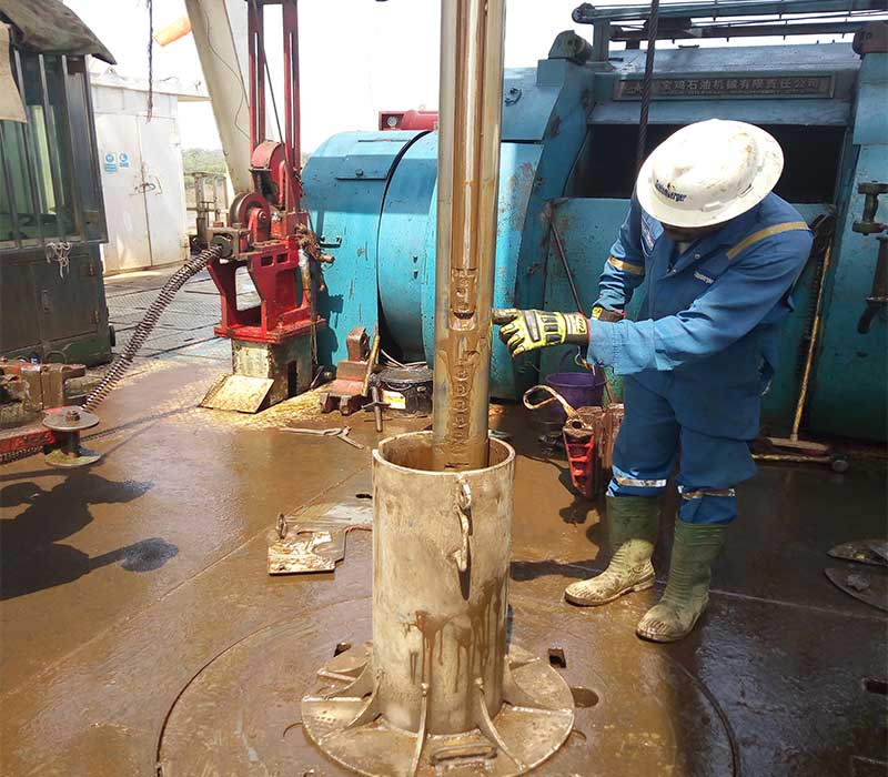
Consultant wellsite geologists, in the oil and gas industry, provide contract services to clients by bringing skill and experience in different perspective of drilling and geology which allows the geology consultant to help companies identify and solve several different problems.

The Wellsite Geologist effectively supervise geological operations at the wellsite during drilling and acts on behalf of the operating oil company, reporting to the Operations Geologist. The role is also analytical in nature, with geological interpretations used to check that the well is meeting geological targets and also to advise drilling personnel on the geological causes of problems experienced during drilling as drilling equipment and fluids interact with the rocks forming the borehole wall. Early recognition of unpredictable geological anomalies can lead to rapid and cost-effective solutions being applied, making the well safer as well as within budget.

Wellsite geologist

The wellsite geologist (WSG) and the company man (DSV), or drilling supervisor are usually the only oil producing company representatives at the rig. Both are oil company supervisors, but the geologist oversees a few teams while the company man supervises the entire drilling operation.

A Wellsite geologist is an oil company subsurface representative at well site or drilling location. They are involve in geological supervision at the well site

The basic function of wellsite geologist is to analyze drill cuttings obtain by mudloggers while drilling by identification and description of lithology with respect to depth which is an aspect of formation evaluation.

Wellsite geologist is often consultant who offer advice to the oil company and take some decisions in conjunction with the operation geologist at office in town. An example of this is when there is a need to stop drilling for casing or coring operation.

The geologist works under the supervision of operations geologists. They are located in the town offices and are the ones to whom wellsite geologist transmit all their report. Wellsite geologists are the main contact point between the oil rig and the geology and geophysics team in town. We communicate and discuss their intentions, plans and concerns to the teams at the wellsite.

What are the functions of wellsite geologist?

Wellsite geologist are responsible for well site geological supervision and all geological related activities at drilling site. The following are responsibilities of wellsite geologist:

Drill cuttings analysis and description

One of the basic duties is the identification and description of drill cuttings circulating out of the borehole with respect to depth. The description is often standardized and defined by each oil company. The wellsite geologist can classify the rock cuttings, check for evidence of borehole instability and confirm the presence of hydrocarbons.  Drilling cuttings are analyzed and described using a stereoscopic microscope under white reflected light. To help identify the presence of hydrocarbons, a UV Box (Ultraviolet Box) is also used. Hydrocarbons will have a variable, but identifiable, brightness when exposed to ultraviolet light.

Several other tests are performed to carry out the formation evaluation. Such tests involve chemicals such as hydrochloric acid, to detect calcium carbonate content, and phenolphthalein, to detect the presence of cement and differentiate it from the formation.

Drill cutting analysis

Data correlations and decisions

The wellsite geologist analyses and interpret  MWD/LWD data for confirmation of lithology, fluid type (oil, gas. water) and compare data gathered during drilling to prediction from seismic section and offset wells for determination of actual formation tops and reservoir sands to ensure the well is drilling in the formations forecasted for a given depth – deeper or shallower relative to the forecast?

When offset well data MWD/LWD and wireline logs are available to the wellsite geologist, data correlation can be carried out which can help to foresee important events like significant gas changes, drilling breaks and potential hazards which occurred in offset wells. You may find the older offset logs usually printed in paper or in a pdf format. The raw data is usually in a LAS file format, which is the most common for the mudloggers and LWD/MWD services to distribute.

Wellsite geologist need to advise the base office and drilling team on the best course of action in several scenarios. As the field geologist you have the responsibility of advising the team to either carry on or stop drilling. Nowadays this is usually a decision made together with operation geologist at office base in town. One such example is selecting at which depth drilling operations must stop in order to set casing or take a core sample.

Data correlation

Formation evaluation services team supervision

There are a few teams and services which wellsite geologists supervise. These are the mudlogging, MWD and LWD, wireline logging, core handling, micro and nano paleontologists. The geologist performs quality control and assurance of these services and the data they provide. These requirements can change from Oil Company to oil company.

Formation Evaluation Services

Coring operations

The geologist is the key figure at the wellsite for taking decision with the office in town on when to stop normal drilling operations, as we approach coring point. Again, wellsite geologist need to use several correlations logs, drill cuttings , offset mudlogging, LWD data and other formation evaluation methods. When reaching coring point the drilling team starts to pull out of hole to proceed with the coring operation.

During coring operation, Wellsite geologist evaluates the few cuttings coming out of the wellbore while cutting the core. When the core is at surface, geologist take core chips from each meter (3 feet) of the entire core to evaluate the presence of hydrocarbons and to decide if coring operations should continue or stop in order to resume regular drilling operations (usually reaching the Total Depth). We must handle, or supervise the handling, of the core on surface ensuring proper markings and saw cutting as per oil company standards.

Core handling

Casing point determination

The role of the geologist, for this operation, will be similar to the coring point approach as our main focus is analyzes of drill cuttings and correlating data with offset wells and ensure that there are no permeable / porous formations close to the bottom of the hole when we reach casing point, or in the rathole immediately below the casing shoe, as that increases substantially the risk of having losses during the cement job that will be performed after running the casing itself.

Geosteering and Horizontal drilling

Wellsite geologist (depending on the oil producing company) coordinate wellsite Geosteering operation in conjunction with Base Operation Geologist by analyzing and interpretation of real time data (Well inclination, Azimuth, correlation, Lithology, Biostratigraphy, reservoir porosity, formation dip and compare with the pre-drill geological model derived from seismic and offset Well data for decision-making as whether to increase inclination or to place the borehole trajectory higher in terms of TVD or to aim for a series of forward target points coordinates and to maintain direction/angle of inclination required at the bit when target is reached) while drilling horizontal Well.   

Geosteering and horizontal drilling

Reporting

Wellsite geologist have several reports to prepare daily, weekly, and at the end of the well. Some of the daily reports are the Daily Geological Report and the Lithology Log. These reports are updated with geological data, ongoing operations and important events.

There is also an End of Well Report or Final Well Report. This is produced and completed during the course of operations at the wellsite. They are delivered as updates to the operations and petroleum geologists during drilling operations. When drilling operations end these reports continue to be completed in the offices in town. They are updated until the end of all wellsite operations and only end when all the data from the entire well is obtained. Final completion of these reports will be carried out by the onshore geology team or the oilfield geologist, if asked to. There are several software packages available for us and these are usually provided by the oil company. Training on how to use them is one of the geological consultant’s responsibilities. For example, some of these software packages will allow you to produce the lithology logs, composite logs and other types of logs which may be required.

Safety and communication

HSE (Health, Safety and Environment) is a key aspect at the wellsite. The geologist is a leader and sets the example at all times encouraging others to work in safe conditions. Safety is one of the most important aspects of the entire operation.

Communication is also key to the success of the operations. Geologist communicate frequently with both the onshore office and the teams at the wellsite. This can reduce misunderstandings and mistakes. Make your teams feel comfortable enough to ask you anything in case of any doubts.

Talk to us for your upcoming wellsite geology consultancy requirement

We specialize in providing highly experience wellsite geologist to clients of all sizes in the oil and gas industry. Contact us at www.geodatadrilling.com Phone: +234 8037055441


Quantitative Methods of Real-Time Pore Pressure and Wellbore Stability Detection

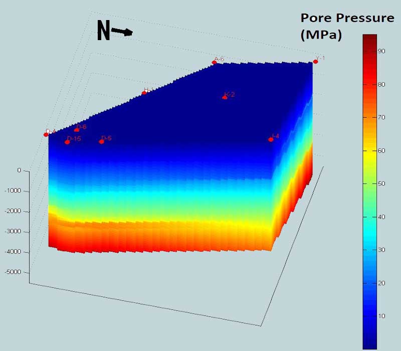
Our pore pressure computer program (Geopressure software)  for detection / analysis of abnormal pore pressures during mud logging (drilling) operation currently supports the following methods:

Overburden gradient calculation

Formation Pressure calculation by:

  • Equivalent Depth Method
  • Ratios Method
  • Eaton Method

Fracture Gradient Calculation by:

  • Eaton Method
  • Daines Method

Shear failure gradient (SFG) or borehole collapse pressure gradient calculation by:

  • Mohr-Coulomb failure criterion

Normal compaction trend line (NCTL) Methods

These are the most common methods in current use, and require a shale sensitive log, a porosity-sensitive log, and an overburden gradient curve corrected for water depth.

  • Compute overburden gradient and correct for water depth
  • Identify the shale points. Select porosity points at the shale points.
  • Determine the normally compacted interval in the porosity-sensitive log and fit it with a normal compaction trend line (NCTL)

Compare each point of the porosity log to the NCTL and compute abnormal formation pressure using an appropriate method.

In practice, fracture gradient also is calculated and plotted with the pressure/overburden curves.

Estimating Overburden Gradient

  • For evaluation of formation pressure
  • For calculation of fracture gradient
API
metric

The Operator can hand-calculate an approximate overburden curve from formation bulk densities for several representative depths over the interval to be drilled. Representative bulk densities may derive from wireline log data, from ‘shale’ (cuttings) densities, or seismic (interval velocity) data.

If we have an electric log for the formation density, we can use it to calculate the overburden:

Divide the log into intervals of depth with similar density.

If the proposed well is offshore, the first two density intervals will be:

  • Air gap between elevation of flowline and mean sea level, with ρb= density of air
  • Water depth between mean sea level and sea bottom (mud line), with ρb = density of sea water.

Then fill the following form to calculate the overburden at the end of each depth interval:

Interval bottom (m)Thickness (m)Bulk density (kg/)Overburden pressure in the interval (kg/cm2)Total overburden pressure (kg/cm2)Overburden gradient (kg/cm2/10m)
1501501.06S=150*1.06/10 = 15.915.9GS= 15.9*10/150 = 1.06
4002501.70S=250*1.70/10 = 42.515.9 + 42.5 = 58.4GS= 58.4*10/400 = 1.46
7003001.8054.0112.41.61
10703701.8969.9182.31.70
      
      
Overburden calculation by depth

Plotting the overburden gradient versus depth gives a curve

overburden gradient vs depth

The equation of the curve is:

S= a(Ln(Depth))2+ bLn(depth) + c

The coefficients a, b and c are regional characteristics

If no density log is available,

a ”hard formation” or a “soft formation” set of coefficients a-b-c is used.

The default coefficients, known as ‘soft’ and ‘hard’ values, were constructed from data for a number of wells in two separate areas:

‘Soft’ coefficients (relatively pure shales)

a = 0.01304

b = -0.17314

c = 1.4335

‘Hard’ coefficients (siliceous shales)

a = 0.01447

b = -0.1835

c = 1.4856

Clients most often prefer to use sonic log densities, or seismic transit times, to calculate formation bulk densities. This set of calculations is known as the AGIP method (Belotti, et al., 1978).

The transit times of sound waves passing through a given formation can be used to define the porosity of the rock, as in the equation below:

Where:

⧍tlog = Transit time reading from the sonic log (μsec/ft)

⧍tm = Rock matrix transit time (μsec/ft)

⧍tf = Transit time of the formation fluid (μsec/ft)

∅ = Porosity (decimal value from 0 to 1)

In practice, the approximate value of ⧍tf is 200 μsec/ft. The values for ⧍tm can be approximated as below

LithologyDensity (kg/l)⧍tma (μsec/ft)  
Dolomite2.8743.5
Limestone2.7143.5 to 47.6
Sandstone2.6547.6 to 55.6
Anhydrite2.9650
Salt2.0267
Shale3*47*
Values of rock matrix and density

Three formulae describe the relationship between porosity and transit times for different types of sedimentary formations.

Consolidated formation
Unconsolidated Sand
Unconsolidated Clay

After approximating the porosity, the bulk density is a function of:

Where:

ρb = Bulk density for the interval, g/cc

ρm = Rock matrix density, g/cc

ρf = Formation fluid density (usually 1.03), g/cc

Requirements for formation pressure/fracture gradient FP/Frac Calculations

For estimated formation pressure calculations, you will need:

  • DCN (‘normal’ trend of compaction increase)
  • Overburden gradient
  • Normal formation pressure (mud density equivalent) or equilibrium density at a specific depth.

For fracture gradient calculations, you will need:

  • Effective vertical stress
  • Tectonic stress (if Daines Method is used)
  • Formation pressure gradient.

Estimating formation pressure Pf

Our Pore Pressure Engineers can calculate formation fluid pressures from any of the following data:

  • Seismic interval velocities
  • Normalized drilling parameters (‘d’ Exponent)
  • Shale density
  • Wireline or MWD logs, including resistivity/conductivity, sonic and direct measurement of downhole pressure
  • RFT/DST (providing direct measurement of pressures)
  • Kick.

In practice, ‘d’ Exponent usually provides the primary pressure data, with the other processes used to verify or correlate the results.

Equivalent Depth Method

We can apply the Terzaghi equation for Overburden pressure, (S= σ+ Pf) . We know that we have the same compaction in A and B, so the stress S must be the same in both points! σA = σB

We can write:

σB =  SB – PfB and σA = SA – PfA

As σA = σB  we have:

SB –PfB = SA –PfA

Thus:

PfA = PfB + (SA -SB)

Overpressure applies the equivalent depth method via the following equation:

  DeqA=Sa –  Hb/Ha * (Sb – DeqB)


Where:

DeqA = Equilibrium density at depth A

Sa= Overburden gradient at depth A

Ha= Depth A

DeqB= Equilibrium density at depth B

Sb= Overburden gradient at depth B

Hb= Depth B

Ratios Method

Application:’d’ Exponent, shale density, wireline/MWD logs(resistivty and sonic log)

Principle:

The difference between observed and ‘normal’ values of a parameter is proportional to the increase in pressure.

As an example, for ‘d’ Exponent, the calculation is:

where:

PF = Formation pressure gradient (mud density equivalent)

H= ‘Normal’ pressure gradient (mud density equivalent)

Eaton Method

Application: Interval velocities, ‘d’ Exponent, wireline/MWD logs(resistivty and sonic log)

The Eaton Method uses the principle that changes in the overburden gradient govern the ratio between the observed and ‘normal’ values of a given parameter.

Shale Resistivity:

Pf Gradient=OVBG – (OVBG – H)*(RshO / RshN)1.2


With H:  normal hydrostatic gradient

         RshN: Theorical shale resistivity on normal trend (B)

          RshO: Observed value of shale resistivity         (A)

         OVBG: Overburden gradient observed at observed depth

Sonic:

Pf Gradient=OVBG–  (OVBG – H)*( DtN /DtO)3.0


With H:  normal hydrostatic gradient

         DtN : Theorical transit time on normal trend (B)

          DtO : Observed value of transit time     (A)

        OVBG: Overburden gradient observed at observed depth

Formation tests

DST or RFT tests give a direct evaluation of the Pf

Estimating Formation Pressure from Kick

In most kicks, the invading fluid does not enter the drill pipe. Thus, the Shut-in Drill Pipe Pressure (SIDPP) represents the amount by which formation pressure exceeds the hydrostatic pressure of the mud column.

Formation pressure equals the sum of mud hydrostatic pressure (inside the drill pipe) plus Shut-in Drill Pipe Pressure (SIDPP).

metric
API

Calculating Fracture Gradient

Liquid exerts pressure which is equal in all directions.

When solids are subjected to external force, it reacts by distributing internal load called stress -giving to stress ellipsoid.

If loading is perpendicular to eliminatory surface the stress is normal.

If loading is tangential to the eliminatory surface shear stress results.

σ = OVB – PF

Fracture occurs when the stress exceeds tensile strength of the rock.

The pressure in this case is fracture initiating pressure. – FP1

If the pressure is suddenly reduced the fracture closes.

To reopen the existing fracture less pressure required – FP2

A surge may open a fracture, afterwards the mud that was holding the hole may not hold any more. Stress is a pressure force per unit area and acts normal to the selected plane.

Stresses acting at any point can be resolved in to 3 mutually perpendicular stresses.

Stress concept

Maximum – σ1

Intermediate – σ2

Minimum – σ3

Relaxed area : Low topography σ1 is vertical and equal to the weight of the overlying rocks.

σ2 and σ3 are horizontal and normal to σ1 .    σ1 > σ2 = σ3

Extreme case:

Tectonically stressed area : Thrust faults etc. σ3 is vertical and equal to weight of overlying rocks.

σ1 and σ2 are horizontal.

When fracture occurs S3 is overcome.

Fracture Pressure  F = S3= σ3 + PF                 σ3 = K X σ1

F – PF = K X σ1

          K  X (OVB – PF)

( F – PF) / (OVB -PF) = K (Stress Ratio).

Thus K can be calculated after LOT. Values of K differ with depth.

Hence a plot of Depth X K is necessary to get proper value of fracture pressure.

Poisson’s Ratio

Eaton introduced Poisson’s ratio to account for variable overburden gradient.

The ratio of lateral unit strain to the longitudinal strain in a body that has been stressed longitudinally within its elastic limits.

Measure an ability of the rock to deform within its limits.

Fracture Pressure F = [ μ/ ( 1- μ)] σ1+ PF

Consider flat lying stratum of semi-infinite extent and weight of overlying strata is the only source of stress.

σ H = [ μ / ( 1- μ)] σ1         μ = 0.25

= [ 0.25  / ( 1 – 0.25) ] σ1

= 1 / 3 (σ1 )

Calculating Frac: Eaton Method

As described previously, Eaton uses Leak-off Test results to compute Poisson’s ratio; this ratio is then use to determine the corresponding fracture gradient:

The fracture gradient at a specific depth is then calculated as a function of:

Calculating Frac: Daines Method

The Daines Method refines the Eaton calculation by allowing for a variable Poisson coefficient based on rock type drilled, and by introducing a correction factor for tectonic stress.

The basic Daines calculation is:

Frac = σt + σ (μ)/(1 – μ) +    PF ; where σ is vertical effective stress

Data from the first Leak-Off test (in a compacted formation) allows back-calculation of the ratio of superimposed tectonic stress:

σt = Frac –  σ ( (μ  )/(1 – μ)+    PF )

To determine the tectonic stress at the Leak-off Test depth:

σt = Frac- σ’1  X  μ/1 – μ+    P

Where:

σt = tectonic stress

Frac = Formation fracture gradient (mud weight equivalent); determined from leak-off test pressure

σ’1 = maximum effective compressive stress

μ = Poisson’s Ratio, as determined from table on next slide

P = estimated formation pressure gradient (mud weight equivalent).

Daines suggested the following Poisson’s ratios for different lithologies (use the one that most closely corresponds to the rock type at the Leak-off Test depth:

Rock typeμRock Typeμ
Clay0.17 to 0.50Sandstone cont. 
Conglomerate0.20poorly sorted, shaly0.24
Dolomite0.21fossiliferous0.01
Limestone: Shale: 
micritic0.28calcareous0.14
sparitic0.31dolomitic0.28
porous0.20siliceous0.12
fossiliferous0.09silty0.17
argillaceous 0.170.17sandy0.12
Sandstone: kerogenaceous0.25
coarse0.05 to 0.10Siltstone0.08
medium0.06Slate0.13
fine0.03Tuff, glassy0.34

After Daines, Journal of Petroleum Technology, 1982

The maximum effective compressive stress is determined as follows:

σ’1 = S – P

Where:

S = overburden gradient

P = estimated formation pressure gradient (mud weight equivalent).

Indicators from Wellbore Instability

When the mud weight is inappropriate, wellbore instability events occur while drilling, which can help to diagnose the overpressure and to adjust mud weight in real-time drilling operations. Wellbore instability can be classified into two categories:

  • Shear failures
  • Tensile failures.

Shear failures

When the downhole mud weight is less than the shear failure gradient (SFG, or borehole collapse pressure gradient), the wellbore experiences shear failure.  Shear failure is mainly caused by the condition in which the applied mud weight is lower than the SFG. The indicators of shear failures while drilling include hole enlargement (borehole breakout), hole closure, tight hole (overpull), high toque, hole fill after trip, hole bridging, hole pack-off, and hole collapse.

 Some of these indicators may be caused by swelling shale when the water-based mud is used because of the chemical reaction between the mud and the shale formation. Therefore, it needs to identify the causes of the failures.

Here we use a vertical well as an example to illustrate the relationship of wellbore instability and pore pressure. Based on Mohr-Coulomb failure criterion, the minimum mud weight to avoid borehole shear failure can be obtained from the following equation:

Pm  = 1 – sin φ/2 (3σH – σ h – UCS) + pp sinφ   

Where 

Pm  = minimum mud pressure or collapse (shear failure) pressure

 φ = angle of friction of the rock

 UCS = rock uniaxial compressive strength

pp = Pore pressure

σH, σ h = the maximum and minimum horizontal stresses, respectively.

The horizontal stresses are most important parameters for analyzing wellbore stability, which can be obtained from either field measurements or calculations

The equation above shows that the shear failure is directly related to the pore pressure; a higher pore pressure needs a heavier mud weight to keep the wellbore from the shear failure. Therefore, wellbore instability can be used as an indicator of an overpressured formation.

Tensile failure

Tensile failure occurs when the mud pressure exceeds the capacity of the near-wellbore rock to bear tensile stress. If the downhole mud weight is higher than the fracture gradient, the formation will be fractured to create hydraulic fractures (or drilling-induced tensile fractures). Real-time indicators of drilling-induced tensile failures include hole ballooning, drilling mud losses, and lost circulation. Reducing mud weight, adding lost circulation materials (LCM), or applying wellbore strengthening technique are possible cures for the drilling-induced tensile failures.

Procedures of Real-Time Pore Pressure Detection

For real-time pore pressure detection and monitoring, the following steps can be performed:

  • Construct predrill petrophysical and pore pressure model and calibrate the predrill model to offset wells if they are available. The model includes methods of resistivity, sonic, Dxc, and so on. The model should include uncertainties and address drilling challenges and potential issues.
  • Apply the model to the real-time well. It particularly needs to have a calibrated NCT for each method.
  • Connect the model to real-time data (e.g., use Connect WITSML to connect LWD and MWD tools), so that the real-time data can be automatically loaded to the model. The model can then automatically calculate pore pressures based on the NCT using the real-time LWD and MWD data.
  • Compare the real-time calculated pore pressure to downhole mud weight (ESD, ECD); to determine if the mud weight is sufficient, particularly it needs to identify whether or not the mud weight is less than the pore pressure gradient. Only comparing the real-time calculated pore pressure gradient to the mud weight is not enough to conclude an underbalanced drilling status. Therefore, it also needs to combine to other real-time indicators of pore pressures.
  • Adjust the models (mainly NCTs) based on the following data if they are available: real-time pore pressure measurement, well influx, mud pit gains, kicks, mud gas data, mud losses, drilling parameters, and borehole instability events (e.g., cavings, torque, fills, and pack-offs).
  • Alert and inform the rig for action when the pore pressure is lower (underbalanced) or close to the downhole mud weight.
  • Liaise with technical expert group on all issues related to unplanned drilling operations, ECD, and pore pressures.
  • Make postwell knowledge capture and transfer within the appropriate organizations and systems.


The real-time monitoring should ensure that:

  • Pore pressure is continuously monitored and indicators of the abnormal pressures are identified;
  • Real-time pore pressure methods, estimates, and updates are discussed routinely with all involved monitoring parties to provide a consistent interpretation to the rig operations;
  • Abnormal pore pressure events are identified as soon as possible;
  • The abnormal events, including significant observations, changes, or updates in pore pressure estimates, if they are occurring or imminent, need to be communicated to the operations (e.g., operation geologist and drilling engineer) quickly;
  • The appropriate actions of operations (e.g. raising mud weight when the pore pressure gradient is lower than the downhole mud weight) are taken quickly.

Talk to us for your upcoming Pore-Pressure and Wellbore-Stability Prediction requirement

Geodata Evaluation & Drilling LTD. Pore pressure consultant use specialist software to provide pore pressure profiles for your wells which are calibrated to offset well behavior for determination of optimum mud weight window for successful drilling operation. Contact us at www.geodatadrilling.com Phone: +234 8037055441

Pore-Pressure and Wellbore-Stability Prediction for Prevention of Drilling incident

Qualitative Pressure detection

When abnormal pore pressures are not accurately predicted in pre-drill stage or detected in real-time drilling, it may cause serious drilling incidents such as fluid influx to the wellbore, kicks, and even blowouts. Pore pressure analysis mainly includes three aspects, these includes:

1. Pre-drill pore pressure prediction.

  • Regional Geology,
  • Geophysical –Seismic

2. While drilling (Real time) pore pressure detection

  • Drilling Rate
  • ‘d’ exponent, Sigma log
  • LWD (Resistivity, Density, Sonic)
  • Drag and torque
  • Mud pit level, Return flow, Pump Pressure (kick)
  • After Lag Time: Gas, (BG, CG, Pump off Gas) MW (out), Cuttings Shape/Size, Lithology (anhydrite, known marker, etc.), Shale density, Shale factor, Temp (out)

3. Post Well pressure Analysis

  • Wire Line Logs: Resistivity, Density, Sonic
  • Direct Pressure: DST, RFT/MDT

This article will focus on methods of while drilling (real-time) pore pressure detection based on overpressure linked to shale compaction anomaly

Drilling Rate – Rate of Penetration (ROP)

In shale, ROP decreases with depth because of decrease in porosity due to compaction. ROP tends to increase as the bit enters an under-compacted section. ROP depends on: Lithology, Compaction, Differential pressure, WOB (weight on bit), RPM (Rotation per minute), Torque, Hydraulics, Bit Type and Wear.

Factors Affecting ROP

Lithology – Drillability depends on: Porosity, Hardness (Calcareous clays), Plasticity, Abbrasiveness (Accessory minerals, such as siderite), Cohesion

Compaction – Compaction increases with depth. The under-compacted section is indicative of higher porosity. This results in increased drillability.

Differential Pressure – Difference of pressure between mud column and formation pressure. Increase in pressure of mud column decreases penetration rate.

Bit tooth impacts on formation, creating fractures. Further impact deepens the fractures, forming rock fragments.

Bit tooth impacts on formation, creating fractures. Further impact deepens the fractures, forming rock fragments.

Overbalance: Rock fragments are difficult to dislodge because of positive differential pressure. Mud Pressure > Formation Pressure

Underbalance: Rock fragments are forced away from formation face. Formation pressure > mud column

Effects of Overbalance:

  • Slower rate of penetration
  • Formation damage
  • Absence or low recovery of hydrocarbons C2-C5 (gas interpretation more difficult)
  • Problems for E-log interpretation.

Weight on bit – Changes in WOB affect drill rate; size of bit affects weight applied per unit of surface area

Weight on bit – in an inclined hole, apparent WOB recorded at surface is not representative of down hole WOB. The string may rest on the hole wall, reducing down hole WOB.

Weight on Bit – Generally ROP increases with WOB, up to a ‘flounder point’ which can vary with formation consolidation. (Threshold Weight : minimum weight required to start drilling. Unconsolidated rocks come apart just by jet action, Flounder Point : Drilling rate stops rising. Bit teeth become jammed with cuttings. Bit cleaning is less effective).

RPM – Relationship of RPM and drilling rate for a given formation. Increased RPM increase drilling rate.

Torque – Measurement of torque at surface is effect of bit and string (stabilizers etc.) MWD torque measured at the bottom is probably true indication of bit torque. (Increase in torque is balanced by twisting of the string. This shortens the string. Weight on bit decreases. The torque is released. String lengthens, WOB increases. The process keeps on repeating.

Hydraulics – Effect of hydraulics depends on consolidation of sediments under drilling.  Increase in flow rate tends to increase ROP (faster clearing of cuttings from under bit).

Mud properties:

Viscosity: Low viscosity with turbulent flow = more effective cleaning of the bit face.

Water loss: Increased water loss may increase penetration rate by reducing time for mud pressure and pore pressure to reach equilibrium.

Suspended solids: Tend to reduce water loss; may dampen bit impact in some cases.

Bit Type and Wear – most often a consideration when tri-cone rock bits are in use.

  • Change of bit type will result in ROP trend change
  • Tooth wear may result in gradual ROP decrease that masks transition zone
  • Controlled drilling practices may mask transition zone
  • Diamond/PDC bits tend NOT to show ROP changes due to wear.

Various methods have been devised to “normalize” the rate of penetration. These attempt to eliminate the effects of drilling parameter variations and thus measure formation drillability. The simplest and most reliable solution is known as ‘d’ Exponent.

‘d’ Exponent

‘d’ Exponent is based on an empirical relationship between drilling rate, weight on bit, rotating speed and bit diameter, first suggested by Bingham (1964):

R/N = a (W/D)d

R = ROP, ft/min

N = RPM

W = WOB, pounds

D = Bit diameter, inches

‘a’ = lithological constant

‘d’ = compaction exponent

Jorden and Shirley (1966) solved for ‘d’ by introducing constants which would allow the use of standard industry units.

Bingham’s constant ‘a’ was assumed to be 1 (constant lithology) and thus is not included.

Original Jordan and Shirley Equation (API):

        log ( ROP / 60 RPM )

d =   ——————————-

        log ( 12WOB / 106BS )

Where:

ROP = ft/hr

WOB = pounds

BS = Bit Size, inches

Original Jordan and Shirley Equation (metric):

         1.26 -log ( ROP / RPM )

d =    ——————————-

          1.58 -log ( WOB / BS )

Where:

ROP = meters / hr

WOB = tonnes

BS = Bit Size, inches

‘d’ Exponent vs. Compaction Trend

Where lithology is constant, ‘d’ Exponent will represent:

  • the state of compaction (relative porosity)
  • differential pressure

A decrease in ‘d’ while drilling in an argillaceous formation is thus related to the degree of undercompaction and of the associated abnormal pressure.

Note: If measured depth and TVD differ significantly, ‘d’ Exponent should be calculated based on TVD.

Corrected ‘d’ Exponent (dcs)

‘d’ exponent values depend in part on mud density and pore pressure. Any change in differential pressure will thus affect ‘d’ Exponent.

Rehm and McClendon (1971) proposed a correction to account for this effect:

                 NG

dcs = d  ——-

                 ECD

NG = Normal Hydrostatic gradient – ppg (API) or kg/l (metric)

ECD = Equivalent Circulating Density – ppg (API) or kg/l (metric)

Dcs Bit Wear Correction

When rock bits are in use, the ROP tends to slow down because of tooth wear. The dcs can show a false increase, thus potentially masking a transition zone. Bit wear corrections have been developed to account for this effect.

Dcs Bit Wear Correction

The Galle and Woods Method

              1.26 – log [ ( ROP * a P ) / (RPM ) ]

d =     ———————————————

                        1.58 – log (WOB / BS )

a = 0.93 Z2+ 6 Z+ 1

                            0.31(FBW)2+ 3(FBW) + 1

Z = X *        ———————————–  

                                  0.31X2+ 3X + 1

X = (Depth – Initial Depth ) / Bit Run

FBW = final bit wear (initially estimated and later corrected)

P = Tooth wear exponent (.4 to .6 for insert bits, .8 to 1 for tooth bits)

Calculating formation pressure from Dcs

Three methods are commonly used in calculation of pore pressure from Dcs:

1. Equivalent depth method

2. Ratios Method

3. Eaton Method

These are discussed in “Quantitative Methods of Real-Time Pore Pressure and Wellbore Stability Detection”.

Setting ‘d’ Exponent Trend

Trend Line (dcn): line joining dcs points in zones of normal pore pressure.

Formation Pressure is calculated from extent of diversion from normal trend.

  • Set the trend in shale only. Select good clean shale section. Avoid silty, calcareous, pyritic shale
  • Avoid using trend values where drilling conditions exist that affect ROP, such as balled up bit, pump problem, mud loss zones, coring controlled drilling, etc.
  • Upper unconsolidated section should not be considered for trend setting.
  • Once trend is set do not change the slope.

To understand the importance of the trend position, you must know that a calculation of the Formation pressure can be made based on the distance between the Dc curve and its normal trend Dcn. Roughly, the Pf curve is a “mirror image” of the distance between Dc and Dcn.

Correct trend setting

In this case above, we can see that some points of the Pf curve go over the MW curve, but these points correspond to sandy zones, and are not to be considered. Only the red dotted line (passing through the shale points Pf) is important and is used as reference for MW selection.

If the trend is set to the sand reference points (left part of the Dc curve), the formation pressure (Pf) curve is shifted to the left. In this case, the formation pressure will not be calculated accurately and the actual Pf will be over the MW before we can detect it.

Wrong trend setting

Are we sure that a deflection of the Dc corresponds to an overpressure ?

If we have a shale gradually grading to a sand, the Dc will have a deflection towards the left; this can be mistaken for the start of a transition zone. Thus it is important to refer to the lithological column when evaluating the change.

With computerized plotting of Dc, we can introduce a ‘sand line’ cut off to eliminate this effect. Dc values to the left of the cutoff are ignored when pressures are calculated.

DC curve in Shaly sand deflected left

If we compare the lithographic column and the Dc, we note that the trends in the shale and in the sand are parallel, there is only a shift. This shows the importance of the cuttings analysis, which is fundamental for the Dc interpretation.

Other drilling parameters for real time pore pressure detection

  1. Torque increase: The swelling of clay cause a decrease in hole diameter, accumulation of large cuttings or caving on the bit and stabilizers, all these problems are linked to negative differential pressure (MW too low).
  2. Overpull and drag increase : for the same reason that causes  the torque to go up.
  3. Hole filling increase : Caving may fill the hole during tripping.
  4. Pit level increase: In case of kick
  5. Flow output increase : In case of kick
  6. Pump pressure decrease: In case of kick, the annulus is filled with mud and  light fluid (i.e. gas), so the pressure losses in the annulus will be less than with a complete column of mud.

MUD LOGGING LAGGED METHODS OF REAL-TIME PORE PRESSURE DETECTION

Indications from Gas:

  • Connection GAS: A good indicator of an increase of pore pressure is the gas “sucked” from the formation during a trip or a pipe connection (by swabbing).
Connection gas and pore pressure

The problem with this method is that it depends on the velocity of the hook when the string is pulled up; two different drillers will give two different pipe connection gases.

A much better system is to check the “Pump off Gas”: the driller stops the pumps without moving the string, so there is no swabbing. But you lose the pressure losses in the annulus; the equivalent mud weight in hole drops from ECD to MW. In that case, a gas show means that the differential pressure is close to being negative.                             

Check also the gas ratios! If you have more heavy gases (ie C2/C3 is decreasing), you enter a transition zone.

  • Background gas and peaks

Check for a. Lithology, b. ROP, c. Flow d. other aspects

  • Trip Gas

Check swabbing conditions (overpull, balled up bit, etc )

Swabbing: Produced gas that enters hole because of suction. This can occur due to:

1. High viscosity of mud.

2. Balled up bit.

3. Fast rate of pulling out.

4. Collar size too large for the hole.

5. Swelling of clays

6. Insufficient cutting transport.

Surging: Injection effect – mud is pushed into the formation. This can occur due to fast rate of running in, and other aspects as above.

Gas Composition: Increased proportion of heavier gasses in transition zone may be indicative of abnormal Pressure. High pressure in zone permits expulsion of lighter gasses; heavier gas are retained. Light to heavy gas ratio shows decrease. C2 / C3 ratio is often used for the purpose. C2 / C3 ratio decrease indicates over-pressure.

Gas Cut mud:

Mud gas is an important indicator of the abnormal pore pressure in drilling operations, particularly in shale formations because of lack of good methods to measure the pore pressure in the shale. If large amounts of formation gas flow into the wellbore, the downhole mud weight is reduced because of the nature of low density of gas. This is “gas cut mud,” indicating that the actual density of the mud coming out of the hole is less than the density of the mud being pumped into the hole. If the gas influx is large, the gas cut mud can cause a marked reduction of the downhole mud weight, and this could result in a gas kick or blowout. Therefore, the gas cut mud is an important indicator of the abnormal pore pressure. Intermediate circulation should be given to degas mud.

  1. INCREASE IN BACK GROUND GAS (BG ) DUE TO CAVING: Gas in isolated pore spaces of shale is under pressure. In trying to escape it forms curved fractures in the shale near wall of hole. The chip then falls in the hole releasing some gas in the process. This leads to increase in BG.

Hydrostatic pressure of mud column < formation pressure:  increase in BG due to caving and gas diffusion from low permeability beds (poor quality mud cake)

Variations in differential pressure will affect the gas recovered at surface. Low differential pressure (low overbalance) between mud hydrostatic pressure and formation pressure will give high gas reading while high differential pressure (high overbalance) will give low gas reading.

  • Mud Weight : An influx with salted water will make the mud density decrease.
  • Mud temperature: The formation temperature gradient will increase in an undercompacted zone. Measuring mud temperature does not give a precise idea of the formation temperature as all actions at surface (new mud, water adding, mixing, trips) will modify the mud temperature. Remember also that the mud has a cooling effect on the bit!
  • Mud resistivity: An influx with salted water has a good electrical conductivity and so the resistivity decreases.

Mechanism generating cavings under overpressure conditions

General rule is that the insufficient mud weight produces more and larger cuttings. There are generally four types of cuttings—normal cuttings, cuttings from pre-existing fractures, cuttings owing to underbalanced drilling, and cuttings owing to shear failures.

  • Normal Cuttings. If the mud weight is appropriate, that is, higher than pore pressure and collapse pressure but lower than the fracture gradient, the wellbore is in a good condition. In this case, normal cuttings are generated with PDC cutting marks when a PDC bit is used, as shown below
Normal Shale cutting
  • Cuttings from Pre-existing Fractures. In a formation with preexisting fractures or in a faulted section, the rock may have a lower compressive strength and lower fracture gradient. In this case, it may generate blocky cuttings in which the naturally fractured planes may be observed; therefore, mud losses probably occur in the preexisting fractures.
Cutting from pre-existing fracture or faulted section
  • Cuttings Owing to Underbalanced Drilling: If the downhole mud weight is less than the formation pore pressure gradient, the wellbore experiences splintering failure or spalling. In this case, spiky and concaved cavings are generalized, as shown in Figure below.
Splintering or spalling caving
  • Cuttings Owing to Shear Failures: Shear failures cause angular or splintered cavings in the wellbore, a case of lower mud weight than the shear failure gradient. as shown below:
Angular splintered caving

Shale density

Plotting shale density (ie using a microsol) versus depth can show an undercompaction. Direct measurement of shale density can be a primary indicator of undercompaction, but several factors limit its usability in the field.

Methods:

1. Variable Density Column: two miscible liquids are mixed to form a column; calibrated with glass beads of different densities.

2. Dense Liquors: series of flasks with fluids of increasing density.

3. Microsol: measurement of cuttings weight in air and weight in water.

4. Mud Balance: measurement of cuttings weight in air and weight in water.

5. Pycnometer: measurement of cuttings weight in air and weight in water.

Limitations of Shale Density

1. Clay must be consolidated for accurate measurement

2. Accessory minerals, carbonate content influence density:

  • Given shale density 2.28
  • Add water filled porosity 15% + 10% pyrite = Density 2.52

3. Caving -not representative of depth.

4. Water-based mud: smectite group of clays adsorb water from mud.

Thus selection of cuttings is difficult, reducing measurement is not always accurate

Shale density vs depth

Mud losses

Mud losses (indicates that differential pressure is too high). If mud losses or lost circulation is observed, it normally indicates that the applied mud weight is higher than the fracture gradient (excluding mud losses into open fractures or vuggy zones), therefore, it may need to reduce the mud weight. When the hole ballooning (borehole breathing) occurs, it normally indicates that the mud weight is very close to the fracture gradient.

What is Borehole ‘Breathing’?

  • The phenomenon of slow mud losses while drilling ahead followed by mud returns after the pumps have been turned off.
  • Borehole Breathing is also referred to as ‘ballooning’ or ‘loss/gain’.

What causes Borehole Breathing?

  • Generally accepted idea is that the phenomenon of breathing is due to fractures being opened and closed by annular pressure fluctuations resulting from mud circulation and non-circulation. The effect of pressure increase is due to Equivalent Circulating Density (ECD).
  • Lowering of the Fracture Gradient due to use of mud coolers may be a cause of breathing.

Why is it important to recognize breathing?

Borehole breathing has often been mistaken in the field for an influx of formation fluid. This can lead to the wrong decisions being made with very costly consequences.

How do you distinguish between ‘Breathing’ and a Formation Influx?

Mud losses while circulating are required for ballooning to occur. Check for small continuous losses while drilling.

LWD / MWD (Shale Resistivity Log)

Resistivity of shale depends on porosity, fluid content and fluid salinity. Under normal compaction and identical environmental conditions, resistivity of shale increases with depth (less fluid content = less conductivity). Thus an abrupt decrease in resistivity is indicative of under-compaction.

Wire line/ LWD conductivity data is generally converted to resistivity. If conductivity plot is available, it will show increased conductivity in an abnormally pressured section.

LWD / MWD (Sonic Transit Time Log)

Sonic transit time is expressed in microseconds per foot.

Interval transit time is given by the equation:

⧍t = ∅⧍t f + (1 – ∅) ⧍tm

Transit time is small in matrix and large in fluid.

Methane=  650

Water = 170 -220

Oil = 238

Quartz = 55.5

For a given lithology transit time will depend on porosity.

Sonic transit time varies with porosity (except when free gas is present). Transit times are faster in the matrix (approx. 40-55 μsec/ft) than in the pore fluids (200 μsec/ft for water). Thus in a transition zone, average transit time will remain steady or increase.

Talk to us for your upcoming Pore-Pressure and Wellbore-Stability Prediction requirement

Geodata Evaluation & Drilling LTD. Pore Pressure consultants use specialist software to provide pore pressure profiles for your wells which are calibrated to offset well behavior for determination of optimum mud weight window for successful drilling operation. Contact us at www.geodatadrilling.com Phone: +234 8037055441

Methods of killing a well after a kick

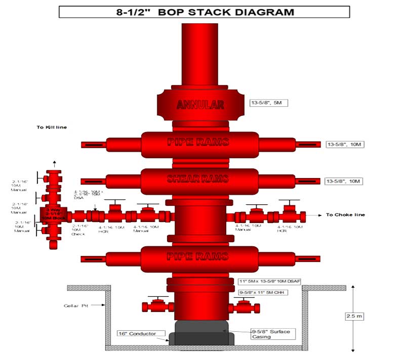
Killing a well or controlling a kick is stopping a well from flowing or having the ability to stop formation fluid (gas, oil or water) to flow into the wellbore. Kill procedures typically involve circulating reservoir or formation fluids out of the wellbore or pumping higher density mud into the wellbore, or both.

What is a Kick

Kick is defined as an undesirable influx of formation fluid into the wellbore. If left unchecked, a kick can develop into a blowout (an uncontrolled influx of formation fluid into the wellbore). The result of failing to control a kick leads to lost operation time, loss of well and quite possibly, the loss of the rig and lives of personnel.

Warning signs of a kick

Warning signs and possible kick indicators can be observed at the surface. Each crew member has the responsibility to recognize and interpret these signs and take proper action. All signs do not positively identify a kick; some merely warn of potential kick situations. Key warning signs to watch for include the following:

Flow rate increase

An increase in flow rate leaving the well, while pumping at a constant rate, is a primary kick indicator. The increased flow rate is interpreted as the formation aiding the rig pumps by moving fluid up the annulus and forcing formation fluids into the wellbore.

Pit volume increase

If the pit volume is not changed as a result of surface-controlled actions, an increase indicates a kick is occurring. Fluids entering the wellbore displace an equal volume of mud at the flowline, resulting in pit gain.

Flowing well with pumps off

When the rig pumps are not moving the mud during flow check, a continued flow from the well indicates a kick is in progress. An exception is when the mud in the drill pipe is considerably heavier than in the annulus, such as in the case of a slug.

Pump pressure decrease and pump stroke increase

A pump pressure change may indicate a kick. Initial fluid entry into the borehole may cause the mud to flocculate and temporarily increase the pump pressure. As the flow continues, the low-density influx will displace heavier drilling fluid and the pump pressure may begin to decrease. As the fluid in the annulus becomes less dense, the mud in the drill pipe tends to fall and pump speed may increase.

Other drilling problems may also exhibit these signs. A hole in the pipe, called a “washout,” will cause pump pressure to decrease. A twist-off of the drillstring will give the same signs. It is proper procedure, however, to check for a kick if these signs are observed.

Improper hole fill-up on trips

When the drillstring is pulled out of the hole, the mud level should decrease by a volume equivalent to the removed steel. If the hole does not require the calculated volume of mud to bring the mud level back to the surface, it is assumed a kick fluid has entered the hole and partially filled the displacement volume of the drillstring. Even though gas or salt water may have entered the hole, the well may not flow until enough fluid has entered to reduce the hydrostatic pressure below the formation pressure.

String weight change

Drilling fluid provides a buoyant effect to the drill string and reduces the actual pipe weight supported by the derrick. Heavier mud have a greater buoyant force than less dense mud. When a kick occurs, and low-density formation fluids begin to enter the borehole, the buoyant force of the mud system is reduced, and the string weight observed at the surface begins to increase.

Drilling break

An abrupt increase in bit-penetration rate, called a “drilling break,” is a warning sign of a potential kick. A gradual increase in penetration rate is an abnormal pressure indicator, and should not be misconstrued as an abrupt rate increase.

When the rate suddenly increases, it is assumed that the rock type has changed. It is also assumed that the new rock type has the potential to kick (as in the case of a sand), whereas the previously drilled rock did not have this potential (as in the case of shale). Although a drilling break may have been observed, it is not certain that a kick will occur, only that a new formation has been drilled that may have kick potential. It is recommended when a drilling break is recorded that the driller should drill 3 to 5 ft (1 to 1.5 m) into the sand and then stop to check for flowing formation fluids. Flow checks are not always performed in top hole drilling or when drilling through a series of stringers in which repetitive breaks are encountered. Unfortunately, many kicks and blowouts have occurred because of this lack of flow checking

Cut mud weight

Reduced mud weight observed at the flow line has occasionally caused a kick to occur. Some causes for reduced mud weight are: Core volume cutting, Connection air, Aerated mud circulated from the pits and down the drill pipe

Fortunately, the lower mud weights from the cuttings effect are found near the surface (generally because of gas expansion), and do not appreciably reduce mud density throughout the hole. 

An important point to remember about gas cutting is that, if the well did not kick within the time required to drill the gas zone and circulate the gas to the surface, only a small possibility exists that it will kick. Generally, gas cutting indicates that a formation has been drilled that contains gas. It does not mean that the mud weight must be increased.

Primary well control

Primary well control is the process of maintaining hydrostatic pressure in the wellbore greater than the formation pressure being drilled, but less than formation fracture pressure. If hydrostatic pressure is less than formation pressure then formation fluids will enter the wellbore. If the hydrostatic pressure of the fluid in the wellbore exceeds the fracture pressure of the formation then the fluid in the well could be lost. In an extreme case of lost circulation the formation pressure may exceed hydrostatic pressure allowing formation fluids to enter into the well.

Secondary well control

Primary well control failed when the hydrostatic pressure in the well (i.e. drilling mud) fail to prevent formation fluids from entering the wellbore. Therefore, a secondary well control is introduced with special equipment called “Blow Out Preventer” or BOP to control unwanted formation fluids in the wellbore.

Choke manifold (Source: Cameron Iron Works)

In order to control a kick, mud of the required density must be added and circulated while back pressure is maintained against the formation. This excess pressure must be slightly higher than the pressure of the fluids contained in the pores of the formation.

There is therefore a need for a line, the choke line, between the annulus and a manifold which directs the effluent to one of the following, depending on the type of fluid involved: mud tanks, degasser, flare, reserve pit

Methods of killing a well

Common circulating well methods of killing a well or well control techniques are:

  • Driller’s method
  • Wait and Weight
  • Concurrent

These all use the same procedures and only differ when and if a kill weight fluid will be circulated.

  • Volumetric Method & Lubricate and Bleed
  • Reverse Circulation
  • Bullheading

The Driller’s Method Procedure

Annular Preventer
  • Shut-in well after kick: Close the annular preventer of Blow out Preventer (BOP). Open HCR valve (Hydraulically control remote valve) to the choke manifold.
  • Record kick size and stabilized shut in drill pipe pressure (SIDPP) and shut in casing pressure (SICP).
  • As soon as possible start circulating original mud (fluid) by gradually bringing the pump up to the desired kill rate while using the choke to maintain constant casing pressure at the shut-in value.
  • Pump pressure should be equivalent to calculated initial circulating pressure (ICP). If not equivalent, investigate and recalculate if necessary.
  • Maintaining pump pressure equal to ICP, kick/influx is circulated out of the well, adjusting pressure with choke as required. After Kick Circulated Out –Killing The Well:
  • Continue to circulate from an isolated pit or slowly shut down the pump maintaining pressure on the choke (casing) gauge equivalent to the original SIDPP.
  • Avoid trapping pressure or allowing additional influx if shutting back in – Avoid trapping pressure or allowing additional influx if shutting back in.
  • The active system should be weighted up to the pre-determined kill fluid density and circulated in order to regain hydrostatic control.
  • If the well was shut in, startup pump procedures are again used.
  • It is advisable to calculate and use a pressure vs. stroke chart (ICP to FCP – final circulating pressure) to track the kill fluid and changes in circulating pressures.
  • Circulate the kill fluid to the bit/end of string.

After Kick Circulated Out –Killing The Well:

  • Once kill fluid is at the bit/end of string, FCP should be realized.
  • Circulating pressure should be equivalent to the calculated FCP.
  • Maintain constant FCP circulating pressure until the kill fluid completely fills the well.
  • The gain in hydrostatic pressure (HP) should necessitate slowly reducing choke pressure.
  • Once the kill fluid reaches surface, the choke should have been fully opened.
  • Shut down pump and check for flow.
  • Close choke and check pressures.
  • If no pressure is noted, open choke (bleeding any trapped pressure), open BOP.

Wait and Weight Method Procedure

  • Shut-in well after kick. Close the annular preventer of Blow out Preventer (BOP). Open HCR valve (Hydraulically control remote valve) to the choke manifold.

2. Record kick size and stabilized SIDPP and SICP, calculate kill fluid density.

3. Pits are weighted up as other calculations are performed.

4. If there are increases in shut-in pressure, the Volumetric Method should be used to bleed off mud/fluid from the annulus to maintain constant stabilized drill pipe/tubing pressure.

5. Once pits are weighted, start circulating kill weight fluid by gradually bringing up the pump up to the kill rate while using the choke to maintain constant casing pressure at the shut-in value. Remember to hold pump rate constant.

6. Circulating pressure should be equivalent to (ICP) Initial Circulating Pressure. If not, investigate and recalculate ICP if necessary.

7. Follow pressure chart/graph as kill fluid is pumped down the string to bit/end of string.

8. Once kill fluid is at the bit/end of string, FCP should be realized.

  • Circulating pressure should be equivalent to the calculated FCP.

9. Maintain constant FCP circulating pressure until the kill fluid completely fills the well.

  • The gain in HP should necessitate slowly reducing choke pressure.
  • Once the kill fluid reaches surface the choke should have been fully opened.

10. Shut down pump and check for flow.

11. Close choke and check pressures.

12. If no pressure is noted, open choke (bleeding any trapped pressure), open BOP.

Concurrent Method

Sometimes referred to as the Circulate and Weight Method or Slow Weight-Up Method. It involves gradually weighting up fluid while circulating out the kick.

Additional calculations are required when tracking different fluid weights in the string at irregular intervals.

Sometimes, crew members are required to record concurrent method data even if this is not the method intended to be used.

The Concurrent Method Procedure:

  • Shut-in well after kick. Close the annular preventer of Blow out Preventer (BOP). Open HCR valve (Hydraulically control remote valve) to the choke manifold.

2. Record kick size and stabilized SIDPP and SICP.

3. ASAP start circulating original mud (fluid) by gradually bringing the pump up to the desired kill rate while using the choke to maintain constant casing pressure at the shut-in value.

  • Pump pressure should be equivalent to calculated ICP. If not equivalent, investigate and recalculate if necessary.

4. Mixing operations begin and pits are slowly weighted up and each unit of heavier fluid reported.

5. Each interval or unit of increased fluid density is then noted and recorded with the pump stroke count at that time.

  • The change in circulating pressure for the different density is calculated.
  • Once this fluid reaches the bit/end of tubing, circulating pressure is adjusted with the choke by that amount.

6. The kick is circulated out and the fluid in the well continues to be gradually increased.

7. Once the kill fluid is consistent throughout the well, shut down pump and check for flow.

8. Close choke, shut well in and check pressures.

9. If no pressure is noted, open choke (bleeding any trapped pressure), open BOP.

Volumetric Method of Well Control

The volumetric method is a way of allowing controlled expansion of gas during migration

  • It replaces volume with pressure (or vice versa) to maintain bottom hole pressure that is equal to, or a little higher than BHP, and below the formation fracture pressure.

With a swabbed in kick, the volumetric method can be used to bring influx to surface and then replace the gas with fluid in order to return the well to normal hydrostatic pressure. It is not used to weight up and kill the well.

  • Used to control the well until a circulating method can be implemented.
  • Can be used to regain HP if the existing fluid is adequate and gas is allowed to reach surface.

Situations where Volumetric Methods can be used:

  • String is plugged.
  • String is out of the hole.
  • Pumps are not working.
  • String is off bottom.
  • During stripping or snubbing.
  • A shut-in period or repairs to surface equipment.
  • Tubing or packer leak causes casing pressure to develop on production or injection well.
  • A washout in string prevents displacement of kick by one of the circulating methods.
  • In subsea operations only 1 line should be used to prevent gas separation effects.

If casing pressure does not increase 30 minutes after a kick is shut in, gas migration is minimal. This means that the Volumetric Method need not be used. However, if casing pressures continues to increase there is a need to initiate Volumetric techniques.

  • Some basic scientific principles must be understood before using the Volumetric Method:

Boyle’s Law–shows the pressure/volume relationship for gas. It states that if gas is allowed to expand, pressure within the gas will decrease. This is the same concept used by the Volumetric Method in that it allows gas to expand by bleeding off an estimated fluid volume at surface, which results in decreasing of wellbore pressures.

Boyle’s LawP1 V1 = P2 V2

Single Bubble Theory–The biggest misconception in well control schools is that the gas enters the well as a “single bubble”.

  • In reality it is dispersed as pumping and observance of the kick is noted, then more “pure” kick as the pumps are shut down and well is shut in.
  • It may be many minutes before the kick is actually noted resulting in an annulus filled with influx/regular fluid.
  • So, in reality, a single large kick rarely occurs, and once the well is shut in, the pressures on the casing shoe/weak zone have probably reached it’s maximum.
  • This is not to say that MAASP should not be observed, just that it should be considered that the maximum pressure should be based on the latest pressure test of the BOP or casing.

Stripping/Moving Pipe and Volumetric Considerations

A stripping pressure schedule must be created in order to control pressures during stripping operations while gas is migrating, pipe is moving, and fluid is being bled off at choke.

Lubricate & Bleed (Lubrication)

 The Lubricate & Bleed Method is used when kick fluid reaches the wellhead.

 It is considered a continuation of the Volumetric Method.

 Generally, workover operations more commonly use the Lubricate and Bleed technique because circulating ports in the tubing are plugged, sanded tubing, or circulation is not possible.

Lubricate & Bleed (Lubrication)

 In this method, fluid is pumped into the well on the annulus side.

 Enough time must be allowed for fluid to fall below gas.

 Volume must be precisely measured so hydrostatic pressure gain in the well can be calculated.

 This value increase will then be bled off at surface.

Reverse Circulation Method of Well Control

 Reverse circulation is the reversal of normal circulation or normal well kill pump direction.

 In reverse circulation, due to friction (APL, ECD) most of the circulating pump pressure is exerted on the annulus.

 Standard start up procedures apply.

Advantage

1. It is the quickest method of circulating something to the surface.

2. Gets the problem inside the strongest pipe from the beginning.

3. Generally, the annular fluid is dense enough to maintain control of the formation, which reduces fluid mixing and weighting requirements.

Disadvantage

1. Higher pressure is placed on formation and casing.

2. Excessive pressure may cause fluid losses/casing and/or formation failures.

3. Not applicable for uses where plugging of circulating ports, bit nozzles of string are possible.

4. Gas filled or multiple densities in tubing may present problems establishing proper circulating rates.

Bullheading Method of Well Control

 Bullheading, or deadheading, is often used as a method of killing wells in workover situations.

 Bullheading is only possible when there are no obstructions in the tubing and there can be injection in the formation without exceeding pressure restraints.

 Bullheading involves pumping back well fluid into the reservoir, displacing the tubing or casing with a good amount of kill fluid.

Complications can make bullheading difficult in certain situations:

– Sometimes, when bullheading down the tubing, pressure may have to be exerted on the casing in order to prevent the tubing from collapsing. Both, tubing and casing burst/collapse pressures, should be known and not exceeded.

– Formation fracture pressure may have to be exceeded due to low reservoir permeability

– Gas migration through the “kill fluid” can pose a problem. In this situation, viscosifiers should be added to the kill fluid to minimize the effect of migration.

Bullheading Procedure

1. Well is shut in and formation pressure is calculated. If bullheading down the tubing, maximum pressures should be calculated.

2. Prepare a rough pressure chart of volume pumped versus maximum pressures at surface. Friction and formation pressure must be overcome to achieve injection of the liquid in the tubing back into the formation. If pressures or pump rate is too high, damage to the formation may occur.

3. Once the pumped liquid reaches the formation, an increase in pump pressure may occur. This is due to a non-native fluid injected to the formation.

4. Once the calculated amount of fluid is pumped, shut down, observe pressures. If no pressure increase is observed, bleed off injection pressure and, again, observe. If no pressure change is seen, the well should be dead. Proceed operations with caution.

Pressure and overpressure formation in Well Drilling

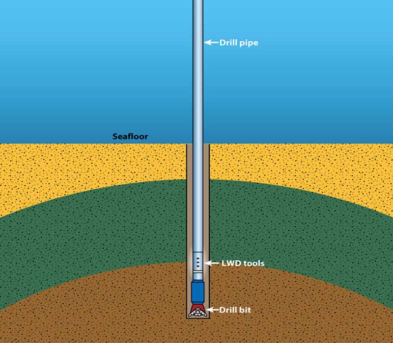
What is pressure?

A pressure is a force divided by the surface where this force applies.

Pressure Pascal = Force Newton / Surface m2

The official pressure unit is the Pascal

It is a very small unit:   1 Pascal = 1 Newton/m2

1 bar = 105 Pascal

1 atm = 1,013 *105 Pascal

A practical unit on the rig is the kgf/cm2

1 kgf/cm2 = 0.981 bar

In API , the unit is the pound per square inch (psi)

1 bar = 14.4988 psi

Hydrostatic Pressure: Ph

Pressure exerted by the weight of a static column of fluid. It is a function of fluid specific gravity and of vertical height of the fluid.

Ph = d * g * H

With    Ph = hydrostatic pressure (Pascal)

            d = Fluid specific gravity (kg/m3)

            H = Vertical height of fluid (m)

Using well site units, the formula becomes:

Ph =   H*d

               10

With Ph= hydrostatic pressure (bar or kg/cm2)

            d = Fluid specific gravity (kg/l)

            H = Vertical height of fluid (m)

Note: The term 10 is approached, for precision, you should use 10.2 with pressure in bars and 9.6 for pressure in kg/cm2

In API, the formula is: Ph = 0.052 * H * d

With    Ph= hydrostatic pressure (psi)

            d = Fluid specific gravity (ppg)

            H = Vertical height of fluid (ft)

Overburden: S

At a given depth, the overburden is the pressure (applying on fluids) or stress (applying on matrix) exerted by the weight of the overlying sediments.

S = H * b

10

With    S = Overburden stress (kg/cm2)

                 b = Formation average bulk density (no unit)

H = Vertical thickness of overlying sediments (m)


In API, the formula is:

S = H * b * 0.433

With    S = Overburden stress (psi)

          ∂b = Formation average bulk density (no unit)

H = Vertical thickness of overlying sediments (ft)

The bulk density of sediment is a function of the matrix density, the porosity and the density of the fluid in the pores.

b= (Φ * f) + (1-Φ) * m

With    ∂b = Bulk density (no unit)

           ∂f = Formation fluid density (no unit)
           Φ = Porosity (from 0 to 1)
           ∂m = Matrix density (no unit)

With depth, the sediment porosity will decrease under the effect of compaction (proportional to overburden) and of course, the bulk density will increase.

You will note that the porosity shale curve is exponential

FORMATION PRESSURE: Pf

Also called Pore pressure: Pp. Is Pressure of the fluid contained in the  pores of the sediment

NORMAL Pf:  Pf=Ph

The formation pressure (Pf) equals the hydrostatic pressure (Ph) due to the column of fluid in the sediment. It depends on the density of the water (usually from 1.00 to 1.08)

NEGATIVE Pf ANOMALY: Pf<Ph

In the following example, the outcrop is lower than the point where the well enter the formation. The water does not reach this zone.

POSITIVE Pf ANOMALY: Pf>Ph

Artesian well: In this case:

Pf = H*d /10     instead of         h * d / 10

Hydrocarbon column

Due to the difference of densities between water and hydrocarbons, the pressure at the top of the reservoir is almost the same that at hydrocarbon –water contact

The formula for the pressure anomaly (excess of pressure respect to normal) is:

Phc = H * (dw – dhc)

                           10

With

Phc = Pressure anomaly at the top of the hydrocarbon column (kg/cm2)

 H  =  Height of the hydrocarbon column (m)

dw = Water SG (kg/l)

dhc = Hydrocarbon SG (kg/l)

Note that this anomaly is proportional to the height of the hydrocarbon column and to the difference of SG between water and hydrocarbon.

Pressure & mud weight

Equilibrium & equivalent mud weight

Equivalent Mud weight is the MW corresponding to a mud column pressure, related to depth. It represents the average mud weight needed to counterbalance formation pressure Pf

From the hydrostatic pressure (Ph) formula, we can recover:

MW = P * 10

             H

PRESSURE GRADIENT: G

A pressure gradient G is the unit increase in pore pressure for a vertical increase in depth unit, but to get consistency with mud weight, we will take 10m.

It is used to give a degree of consistency to pressure data: Pressure gradient and mud weight will be comparable. As the figures are similar, MW and Pressure gradient may be plotted on the same graph, allowing a comparison between MW, Formation pressure gradient, Fracture gradient (fracture pressure gradient is the pressure required to induce fractures in rock at a given depth) and Overburden gradient.

As the figures are similar, MW and Pressure gradient may be plotted on the same graph, allowing a comparison between MW, Formation pressure gradient, Fracture gradient and Overburden gradient.

Stress Concept

Unlike liquids, solids can withstand different loads in various directions: Imagine a cube of porous rock somewhere in the deep. We can divide the stresses in 3 resulting forces according to the 3 directions of space: S1 can be considered as the Overburden , S2 and S3 the tectonic forces (open hole ovalization can give an idea of the difference between S2 and S3).

In a porous rock, the fluid may support part of the stress (due to undercompaction) and the total stress S will have 2 components:

S = Pp +   (Terzaghi equation)

With  S   = Total stress (kgf/cm2)

Pp = Pore pressure ( or formation pressure) (kgf/cm2)

 = Effective stress (on the grains of the rock) (kgf/cm2)

Consequently:

S1 = Pp + 1

S2 = Pp + 2

S3 = Pp + 3

So, in theory, the formation pressure is limited by the overburden !

Origins of Abnormal Pore Pressure or Overpressure Formation

1. Under compaction (overburden effect)

The main cause of overpressure formation.

Normally, the compaction increases with depth and the formation water is expelled as the porosity decreases. In some cases, the water cannot be eliminated in time and remains trapped in the sediment: the main cause of overpressure is due to what is called undercompacted shales. Water elimination from shale depends on 3 factors:

  • Clay permeability: very low
  • Sedimentation and burial rate: if the sedimentation rate is very high, the shale is brought very deep before the water has time to go and it remains trapped in the sediment (ie: deltaic areas)
  • Drainage efficiency: sand layers act as a drain and helps water elimination, less than 15% of sand content in a shale will cause a lack of drainage and an overpressured zone.

Terzaghi experiment

The springs represent the matrix, and the load on the upper plate represents the overburden.

A: the lower tap is closed (no drainage) and S is only supported by the fluid:

S = Pf

B: The lower tap is open, water escapes and the spring/matrix bears part of the load: At that stage, if you close the tap, you get something similar to an undercompacted shale: the fluid is trapped in the sediment and supports part of the overburden, causing an overpressure.

S = Pf + ☌

C: The springs/matrix fully support the load: this is the case of a normally compacted sediment.

Pf = Ph

S = ☌

2. Aquathermal expansion

The volume of water increases with temperature, if it is in a sealed environment, its pressure increases. (Actual effect is controversial.)

3. Clay diagenesis

With depth, the smectites (as Montmorillonite) will lose its adsorbed water and transform into Illite with free water. (Not really a cause of overpressure, but acts as a contributory factor in case of under-compacted shale)

4. Osmosis

Osmosis is the spontaneous movement of water through a semi-permeable membrane separating two solutions of different concentrations, until the concentration of each solutions becomes equal.

A clay bed can act as a semi-permeable membrane between two reservoir containing water with different salinity. ( Note: Not proven in nature and anyway minor effect if exists.)

5. Evaporites

Sealing role: Evaporites are impermeable and can make a good seal that will block water expelled from underlying sediment, creating overpressure by overburden effect. (Note: Major role in overpressure generation, specially if interlayed with shale.)

6. Sulfate diagenesis

Gypsum is the precipitated form of CaSO4, transformation to Anhydrite may occur early in the burial process:

CaSO4,2H2O (Gypsum) D  CaSO4 (Anhydrite) +2H2O

The water amounts to 38% of the original volume, if it cannot be expelled, overpressure develops. Similar increase of volume is created by rehydration of Anhydrite. Note: Minor effect as the diagenesis of gypsum to anhydrite often occurs at shallow depth, this allows the water to escape. Rehydration of Anhydrite is not proven on a scale that would be enough to generate overpressure. 

7. Organic matter transformation

At shallow depth, bacteria will transform organic matter into biogenic methane. From a depth of 250m, thermochemical cracking will transform heavy hydrocarbons to lighter ones, with increase of volume. If these processes occur in a close environment, they create overpressure. Note: Important role in overpressure generation in confined series of shaly sands or carbonate.

Tectonics

8. Relief & structuring

Relief can be the cause of pressure anomalies (ie: artesian well). An artesian well is simply a well that doesn’t require a pump to bring water to the surface. This occurs when there is enough positive pressure in the aquifer to bring the water to the surface. An artesian aquifer is confined between impermeable rocks or clay which causes this positive pressure.

9. Re-organisation of stress field

Sediments are subjected to overburden and to horizontal tectonic stresses.

10. Faults

Faults can create a seal and stop the water or on the contrary, bring an overpressured zone in front of a permeable zone, allowing the water to escape

11. Carbonate compaction

Normally, carbonates do not have problems of undercompaction. Chalk is the exception. Chalk is  due to the deposit of tiny discs called coccoliths (calcareous plates protecting some phytoplankton) and Chalk structure looks like Clay structure, with the same problem of low vertical permeability.

 12. Permafrost

Typical of the artic zones. The overpressure is due to unfrozen pockets (called taliks) inside the permafrost. If a talik freeze, its volume tends to increase (remember that ice is bigger than original volume of water), but the permafrost impedes expansion, thus creating overpressure.

How to describe Drill Cuttings for Oil and Gas well drilling

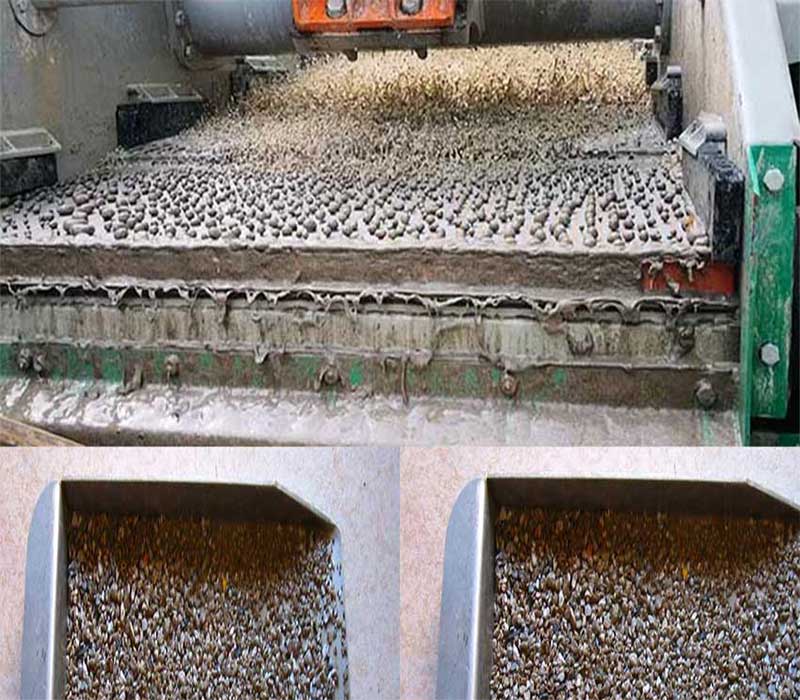
Cuttings descriptions should be done in a consistent order, thus minimizing the chance of missing something out. A conventional order is laid out below, although some operating companies have peculiarities of their own. The common rocks found while drilling oil wells can be split into three categories, namely:

a) Claystone and Siltstone

b) Carbonates and Evaporites

c) Sandstone

Drill cuttings can be group into Clastic, Carbonates and Evaporites:

Clastic

Clastic sediments are sediment consisting of fragments of rock, transported from elsewhere and redeposited to form another rock. (Claystone, Siltstone and Sandstone).

Carbonates

Carbonates are rocks composed of lime mud and/or biogenic debris (shell fragments, algal structures etc.), or their recrystallisation products.

Evaporites

Evaporites are rocks deposited either by the direct evaporation of a body of water, or by a continuous process, whereby minerals are deposited at or near a terrestrial surface, as water evaporates from that surface.

The method of description varies slightly for each category.

Claystone and Siltstone

a) Rock Name Self explanatory but be aware that what looks like a Siltstone, is often a micromicaceous Claystone

b) Colour Colour or combination of colours (e.g. pinkish brown) can be used with qualifiers such as pale, light or dark.

c) Hardness Typical terms used are: Soft, Firm, Moderately Hard, Hard. These have specific meanings. Soft grains offer no resistance to the probe when prodded. Firm grains break apart easily, Moderately Hard grains break with some difficulty. Hard grains are difficult to break at all, and tend to fly out from under the probe. Brittle is sometimes used, particularly when describing Coal or Salt, to describe relatively hard rocks that break easily along fracture planes.

d) Break A term used to describe the morphology of the cuttings. Examples are Blocky (breaking into rectangular fragments), Angular (majority of corners are less that 90°), Splintery (pointed, elongated cuttings), Fissile and subfissile (having more or less well-developed laminar or platy structure). Amorphous means having no form, and is commonly used to describe soft cuttings.

e) Swelling This describes the tendency of cuttings to absorb water over a period of time. It is notoften described in oil based muds as oil on the cuttings surface can affect  absorption. Conversely, washing with detergent sometimes gives an over enthusiastic reaction. Common terms used are Hydro- or Hygroturgid (swelling in a random manner), Hygrofissile (swelling into small flakes) and are usually qualified by ‘slightly’, moderately’ or ‘very’. The term Cryptofissile may be used, this describes a similar reaction to hygrofissile but induced by 10% HCl.

f) Modifiers Not all rocks are composed of one grain type. Argillaceaous is used with non-Claystones with recognisable clay content. Similarly the terms Silty and Sandy can be used. (Arenaceous is interchangeable with Sandy)

g) Carbonate content: Calcareous with the qualifiers ‘Non’, ‘Slightly’, ‘Moderately’ or ‘Very’ describe the way in which a cutting reacts in 10% HCl. Dolomitic is used to describe a cutting that reacts only after several minutes immersion or after warming. Be aware that oil based mud residue also inhibits reaction times therefore cuttings should be crushed to expose fresh surfaces.

h) Accessories These are the small quantities of other minerals present in the major lithology. Examples are Pyrite (which may be described as disseminated i.e. fine grains scattered throughout the rock, or nodular i.e. a crystalline mass), Glauconite, Mica, (which may be prefixed with micro to describe the fine disseminated form.) and Carbonaceous. The usual qualifiers of quantity can be used with these minerals (i.e. ‘slightly’ etc.); also used are common, locally (specific to some horizons) and occasionally (scatted randomly throughout).

Drill cuttings under the Microscope

Carbonates and Evaporites

Carbonates are rocks composed of lime mud and/or biogenic debris (shell fragments, algal structures etc.), or their recrystallisation products. Evaporites are rocks deposited either by the direct evaporation of a body of water, or by a continuous process, whereby minerals are deposited at or near a terrestrial surface, as water evaporates from that surface. Both Limestone and Gypsum/Anhydrite are prone to conversion to Dolomite after burial, when subjected to Mg rich ground waters. In the Zechstein sequence of the Southern North Sea, intergrown masses of Anhydrite and Dolomite are commonly seen, in which it is difficult to determine the dominant constituent. Care must be taken when washing samples containing salts to avoid dissolving the cuttings. It often best to wash them with base oil only.

a) Rock Name Self-explanatory. Identification of more obscure evaporite minerals can be difficult. Most Calcium Sulphate is Anhydrite at bottom hole temperature and pressure, but tends to hydrate due to bit and mud action.

LIMESTONE, DOLOMITIC LIMESTONE, CALCITIC DOLOMITE, DOLOMITE

This can be determined by placing a few grains of the carbonate into a miniature test tube, in practice it is usually carried out on the watch glass, adding a few drops of 5% Hydrochloric Acid.

Hydrochloric Acid Reaction

Limestone (90-100% CaCO3) Instant violent reaction, specimen dissolves within approximately 5 minutes

Dolomitic Limestone (50-90% CaCO3) Moderate but continuous reaction

Calcitic Dolomite (10-50% CaCO3) Weak initial reaction but accelerating after a few minutes

Dolomite (<10% CaCO3) Hesitant. Beads slowly forming during up to half an hour

Alizarin Stain Test

Also, there is a chemical test which can be carried out to determine the presence of the Ca++ ion. This is known as the Alizarin Stain test and takes just a minute or so.

The mudlogging unit should have a supply of the reagent made up. The reagent is added to a miniature test tube containing a few pieces of the carbonate. After a minute, check the colour of the cuttings.

If they are pure calcite ie. Limestone, the cuttings are stained red, if they are pure dolomite, the cuttings are unstained.

EVAPORITE

Rock Type  Identification
Na-Salt – HALITE (Rock Salt):Soluble – recognizable by taste
K-Salt (Potassium salt):Very soluble – has a bitter taste
Mg-Salt (Magnesium salt):Extremely soluble – it feels like is effervescing or prickling on the tongue.
GYPSUM:Turns white if held over a flame (also floats on bromoform).
ANHYDRITE:Remains clear if held over flame (sinks in bromoform) It should be possible to recognize three different types of anhydrites.
Identification of Evaporites

a). Bedded Anhydrite – which is usually white or lightly colored and translucent to opaque. Often is possible to see bedding in cuttings samples

 b). Void filling Anhydrite – transparent crystal with well-defined cleavage

 c). Replacement Anhydrite – lightly coloured and translucent to brown in colour

Tests for Evaporites Minerals

MethodAnhydriteGypsumCalcite
Reaction with Hydrochloric acidNo ReactionNo ReactionViolent Reaction Production of CO2
Barium Chloride Test (note1)White Precipitate of barium sulphateWhite Precipitate of barium sulphateNo Reaction
Density: using Bromoform s.g 2.90Anhydrite s.g. 2.9 to 2.98 – sinksGypsum s.g. 2.31 to 2.32 – floats 
Polarizing Microscope (note2)Right-angled cleavage, marked polarization tintsSlight refractivity grey to whitish tints 
Test for Evaporites

NOTE 1 dissolve in dilute boiling HCl for 5 mins; add a few drops of a normal BaCl2 solution.

NOTE 2 grind sample moderately fine and place a few grains in a drop of water on a slide, cover with a cover slip.

PROBLEMS

There are a number of problems that may arise for the geologist when describing cuttings whilst drilling evaporite sequences.

If you are drilling the section with a salt saturated mud system to reduce washouts, drilling fluid salts may precipitate out and appear at the shakers. Check with the mud engineer. Remember to keep fresh samples of mud chemicals in the mudlogging unit.

As Na- K- MG- salts are very soluble it is often difficult to evaluate the percentages of salts to anhydrite in samples taken from the shakers. Obviously, the samples should not be washed in water until salt proportion has been estimated. However, if drilling salt and anhydrite, the ROP will help as anhydrite drills slower (much slower) than salts and slower usually than carbonates.

Anhydrite often reaches the surface as a soft white paste which may wash through even fine sieves. Also, the Anhydrite may become hydrated in the mud column and you may see it as gypsum in the sample. So, what appears as Gypsum may in fact be Anhydrite in the formation. Gypsum is unstable below about 2500 feet however and loses water to the formation, becoming Anhydrite.

NOTE: Wellsite geologist should determine casing point at competent formation to set casing before drilling through evaporites intervals.

An example Anhydrite description follows:

ANHYDRITE: White, opaque to translucent, occasionally colourless and transparent, hard, cryptocrystalline, with rare thin very light grey Limestone laminations, nil visible porosity, no shows.

An Example Salt description also follows:

HALITE: colourless and transparent to very light brownish grey, transparent to

translucent, firm, brittle, crystalline, locally grading to K-SALT: moderate reddish orange, hard, brittle, crystalline to locally amorphous, with rare thin dark reddish brown saliferous CLAYSTONE laminations.

b) Colour In addition to the terms outlines above, some minerals are described as Colourless. These, and some coloured minerals, also allow the transmission of light and can be further described as Transparent (clear) or Translucent (semi-opaque).

c) Hardness As above.

e) Break As above.

f) Texture This is used to describe the internal structure and or composition of the cuttings. Terms used include Microcrystalline (having a crystal structure that is not visible except under the higher power lenses of the microscope), Crystalline (having an easily seem crystal structure), Cryptocrystalline (crystalline in appearance but having no visible structure, commonly applied to Chert). Sucrosic can be used to describe a fine-grained rock that has a sugary appearance. Texture in Limestones can be described using Dunham’s classification (Wackestone, Packstone etc.) which can be found in manuals and is based on the proportions of lime mud to skeletal fragments. The term Oolitic may also be used when Limestone contains spheroids of algal origin.

An example of a limestone description may be seen below:

LIMESTONE: Bioclastic Wackestone, yellowish grey to light greenish grey, fine to medium grained, firm to moderately hard, brittle, blocky, chalky in places, with occasional dark greenish grey Claystone laminations, rare very fine pyrite cubes, locally pitted, trace disseminated carbonaceous material, trace visible intergranular porosity, no shows

An example dolomite description also follows:

DOLOMITE: Sucrosic, brownish grey, hard, brittle, traces of bivalve fragments, fair visible intercrystalline primary porosity, good to excellent inferred vuggy porosity (from loose medium to coarse dolomite crystals), no shows.

PARTICLE TYPE

If this is discernable in the sample, using Folk’s classification.

SKELETAL PARTICLES – Bioclasts, describe and qualify if possible

NON-SKELETAL PARTICLES – Pelletoids

COATED PARTICLES – Ooids, Pisoids, Onkoids

AGGREGATES OF PARTICLES – Grapestone, Onkolites, Stromatolites

f) Modifiers Limestones can contain significant quantities of sand or clay and are describes as Argillaceous or Arenaceous respectively. They may also be Dolomitic which decreases the rapidity of reaction with HCl. Halite also commonly contains clay laminations.

g) Accessories As Above. Limestone often contains carbonaceous laminations.

h) Porosity Carbonates may exhibit porosity and should be examined thoroughly. While intergranular porosity may be seen in Oolitic Limestones, the principle type is fracture porosity. Vuggy porosity may also be seen where elements of the original fabric have been leached away by groundwater. Porosity is usually qualified by nil, poor, fair or moderate, good and very good or excellent. The terms visible or estimated are also usually applied, as visually porosity estimation can be very subjective.

i) Shows Although carbonate reservoirs are not commercially important in the UK, they often contain hydrocarbon shows. These should be observed and noted. Be aware that minerals in the carbonates can also fluoresce.

Drill cuttings

Sandstone

The description of Sandstone can be split into two parts, the properties of the whole rock, and the properties of the grains that make up that rock.

a) Rock Name Sandstone or Sand. Sandstone is composed of cemented Sand grains, but be aware that bit action can reduce even reasonably well cemented Sandstone to a tray full of grains. Also be aware that PDC bits can turn well cemented Sandstone into a silica paste often referred to as rock flour. If the cement is calcareous, testing with acid may also give the false impression of drilling Limestone. Look for tell tale grains of sand trapped within the paste.

b) Colour This deals specifically with the colour of the rock.

c) Hardness The term Friable is used in place of soft and firm in the scheme above. Loose is used where only Sand grains are observed.

d) Break In addition to the scheme as outlined above, the term Crumbly is used to describe a cutting of irregular outline.

e) Grains Grain descriptions are split into the following sub divisions: Type Usually Quartz but maybe Feldspar (although this is difficult to distinguish from cuttings alone) or Lithic (a redeposited grain of a pre-existing rock type). The following grain description categories should be applied to each type if they occur in significant quantities.

Colour Grain colour should be described, and an estimate made of light transmission properties (transparent, translucent, etc.). The term Frosted is also used to describe grains with an abraded outer surface; these are commonly found in wind blown sand deposits.

Size Grain size should be measured using a comparitor a known size. Not by guessing!

Roundness Grain roundness is an estimate of the surface smoothing of the grain and is independent of the grain shape.

Sphericity Conversely sphericity is an estimate of the grain shape. Aids to the type of sphericity and roundness are commonly combined on grain size comparitors

Sorting Sorting is a visual estimation of the variety of grain sizes in a Sandstone. This is usually straightforward i.e. if there is little variation then the sample is well sorted. Be aware that some Sandstones consist of well sorted laminated layers of two different grain sizes, but these may appear poorly sorted in a cuttings sample.

f) Cementation Cementation is described both in terms of degree and type. The terms poor, moderate, well, etc., are used to describe the difficulty with which the cement bond can be broken, not the degree to which the pore spaces are filled with cement. The common cement types are silica, calcite and dolomite, but iron oxide, pyrite, anhydrite and rarely barite, may be encountered.

g) Modifiers Once again, Sandstones can contain significant quantities of clay, and the term Argillaceous can be used. Sandstones containing significant quantities of Feldspar are often referred to as Arkosic and those with significant rock fragments as Lithic.

Conglomerate Sandstones are often found, particularly at channel bases in fluvial or sub sea fan systems. While easy to see in cored sections, they are often missed in cuttings, due to the breakup of constituent pebbles by the drill action. Look for angular shards of quartz with one rounded facet.

h) Accessories As previously discussed.

i) Porosity Porosity estimation in cuttings is extremely subjective, principally because, as grainsize decreases, the apparent pore space diminishes. Consequently porosity is  commonly under estimated. Estimates can also be affected by the deposition of drilling fluid residue in the pore space.

Oil Flouroscope

Shows The most important bit last! Does the rock contain hydrocarbons?

Shows should be considered in the following way:

1) Examine the cuttings for oil staining under the microscope.

2) Examine the cuttings under UV light. Describe the colours seen. Colours range from bluish white in condensates through yellow, orange and brown in crude to black in bitumen and dead oil. Be aware that base oil usually exhibits a pale bluish white fluorescence, a comparative sample of the mud filtrate can be kept in the UV box. Oil base mud can invade and flush the formation considerably altering show quality. Pick out some representative cuttings and place them in a spotting tray. Examine these under the microscope and check that they are Sandstone, as some minerals, particularly Calcium Carbonate also exhibit fluorescence.

3) Place the spot tray back in the UV box, and while watching, immerse the cuttings in solvent. Describe the rapidity, character and colour of the hydrocarbon as it is leached from the rock. This gives an indication of the permeability of the cuttings and mobility of the oil. If leaching is very slow, then crush the cuttings and observe the changes in the fluorescence.

4) Describe the colour of the oil stained solvent under natural light. Allow the solvent to evaporate and describe the colour of the residual ring in the tray. Darker colours indicate heavier crudes.

REMEMBER! Describe what you see – not what you think you see!

Talk to us for your upcoming Mudlogging services and wellsite geology consultancy requirement

We specialize in providing mudlogging services and highly experience wellsite geologist to clients of all sizes in the oil and gas industry. Contact us at www.geodatadrilling.com Phone: +234 8037055441

Solid Control and Drilling Waste Management in Oil Well Drilling

Solids control is a technique used in the oil drilling rigs to separate the solids or rock cuttings by the drill bits that are brought to the well surface by circulating drilling mud. When unwanted solids are efficiently removed from the circulation system, the fluids in the wells are of highest quality and predetermined specification. Efficient Solids Control results into less replacement of fluids, less waste and few additives that are needed to be removed and disposed there by cutting the cost of the drilling mud. This also significantly decreases the risk of down hole related problems due to excessive solid contents in the drilling fluid.

When proper Solids Control techniques are used, they can reduce the drilling fluid clean up, maintenance cost, and the disposal cost. The Solids Control system is divided into five stages:

Shale shaker.

Mud tank.

Desander.

Vacuum degasser.

Desilter.

The desander separates sand and silt from drilling fluids, the shale shaker separates big solids and the desilter is used to segregate solids. The desilter and desander can be combined to form one high efficiency mud cleaner. Vacuum degasser is used to separate gas, when gas enters the drilling fluids. When the fluids are gas free, the degasser can be used as a big agitator. All these stages are carried out on top of the mud tank. After solids are separated, the clean mud is again pumped into the well bore.

For proper drilling waste management, additional solid control equipment are provided by Solid control services contractors and these include: Decanter Centrifuge and Vertical cutting dryer

Decanter Centrifuge separate drill cuttings (solids) from the drilling mud in the drum equipment component. The high-speed rotating drum drive drilling mud to rotate speedily and then the mud is thrown onto drum’s surface to form a fluid circle. Under the centrifugal force, solid sedimentary force in the separated liquid will be several hundred even thousands of times heavier than its own gravity so as to separate the solids from the suspension quickly. The ratio of centrifugal force which the solids have gained and the solid gravity are called separating factor. The larger the centrifugal force, the finer the separated solids. Decanter Centrifuge removes solid phase from drilling mud and recover weighting materials such as barite, etc. so as to reduce the general cost of drilling mud fluid

Decanter Centrifuge

Vertical Cuttings Dryer uses centrifugal force to dry drilled solids in oil or synthetic base mud. A stainless steel screen bowl traps “wet” solids and accelerates them up to 900RPM. Liquid is forced through the screen bowl openings, while “dry” solids are extracted by the angled flights attached to the cone, which rotate slightly slower than the bowl. Tungsten carbide protects the flights from abrasive solids and ensures long operational life. This aids in maintaining a constant gap between the scroll and screen bowl, which is crucial for proper operation.

Vertical Cuttings Dryer remove particles below 3mm and reduce the liquid content in cuttings with oil base mud/synthetic base mud up to 3-5%OOC(Oil on Cuttings) to make the discharged cuttings comply with the requirement of environment protection and recover the valuable drilling mud and lower down the drilling mud cost.

Vertical Cutting Dryer

Talk to us for your upcoming Solid Control and Drilling Waste management project

Geodata Evaluation & Drilling Limited offers Solid control and drilling waste management services to Oil and Gas industries. Let us handle the project for you. contact us at www.geodatadrilling.com Phone: +234 8037055441

« Older posts

© 2023 geodata & Drilling

Theme by Anders NorenUp ↑